Open Journal of Marine Science
Vol.2 No.1(2012), Article ID:17066,9 pages DOI:10.4236/ojms.2012.21003
Some Catch-at-Age Analysis Methods and Models Compared on Simulated Data
Marine Resources Section, Marine Research Institute, Reykjavík, Iceland
Email: thg@hafro.is
Received September 19, 2011; revised December 5, 2011; accepted December 12, 2011
Keywords: Stock Assessment; Simulation; AD Model Builder; Integrated Likelihood; Natural Mortality; Random Effects; VPA
ABSTRACT
Estimation of parameters and random effects using true maximum likelihood methods is compared to the commonly used penalized maximum likelihood method. The simulated catch-at-age datasets have all conceivable noise in stock and fishing dynamics in addition to the observation error on the catch. Improvement is modest in simple models but refinements that are only possible with these methods provide additional precision. Unbiased estimation of natural mortality is made possible with these methods, but precision is low unless variation in fishing effort between years is large and other variation small, in particular the uncertainty in the recruitment. Relatively unbiased estimates of all other input parameters and variances were obtained. Alternately the stock may be updated with the catches directly, rather than through the fishing mortality. This can be done exactly and such that bias in the final stock is small. Such a model will test a different error structure and may also be more appealing for presentation of results as the catches are in better agreement with the changes in the estimated stock.
1. Introduction
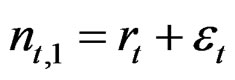
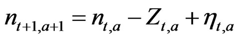
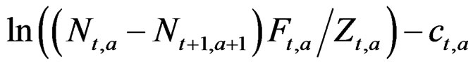
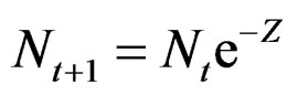
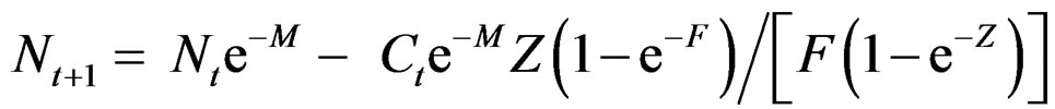
During a review of the assessment modeling of the fish stocks of Iceland several questions on analytical approach came to the fore. In the early Virtual Population Analysis (VPA) work the stock was updated by subtracting the observed catch (C) each year, with a correction for the interaction of the fishing and the natural mortality that may be approximate as in Pope [1,2] but these calculations can also be exact (see appendix). This approach is here referred to as the N – C model. In what is commonly referred to as statistical catch-at-age analysis the stock is updated using the estimated fishing mortality (F) for that fishing season and age class. If the logarithm of the stock ln(N) at a given age is denoted by n then the formula to update n for this age class to the next year is n – Z, where the estimated total mortality (Z) is the sum of the estimated fishing and estimated (or assumed) natural mortality (M) of each age class in each year Z = F + M. This is here referred to as the n – Z model. The effect of the Pope approximation on the selection function has been studied [3] but little attention appears to have been given to the difference in the error structure of these approaches. By using not an approximation but exact N – C calculations (see Appendix), there is no distortion in the selection function so the focus here can be on the effect of the randomness in these two models. In the n – Z model any errors in the estimate of Z will be propagated through the stock equation from one year to the next and show up as correlations in the residuals. This error may be due to fluctuations in the selection by age (S) that do not fit the generally assumed so called separable F = E * S model of fishing effort by year (E) and selection by age, or indirectly due to variation in natural mortality and errors in the observed catch. The N – C model is not directly affected by errors in the estimated Z, but observation errors in the catch will be propagated unmitigated through the stock equation. The errors in reported catch may be due to misclassification by age (generally by age-length-keys), misreporting and gear induced mortality.
With true likelihood methods (integrated likelihood, IL) such as Kalman filter [4,5] it is possible to get estimates of these unobserved internal errors and even correct for them. Earlier modeling of this stock had used the penalized maximum likelihood (PL) method where the point likelihood of both parameters and state variables is jointly maximized simultaneously, but this method has been demonstrated to produce biased estimates and poor precision even when limited to problems where this appears to work [6] and Markov chain Monte Carlo simulations with these methods are of no value in this situation. A recently available public domain statistical package ADMBRE (Auto Diff Model Builder Random Effects) offers a general way of applying the IL method to problems of this kind [7,8] and produces exactly the same results on tested linear time-series problems as obtained with the Kalman filter and in close agreement when applied to simple catch-at-age models assuming normal errors in the observations in log-space.
Another advantage of the IL methods is that certain other variances can be estimated that can not be obtained with direct PL methods, where these variances would have to be assigned some arbitrary fixed values. However in some datasets these errors still do not get estimated (the variance tends to zero) even with these advanced methods. The IL method on Icelandic haddock with catch at age data 1979-2008 and survey data for most of the period could not estimate the variance in the fluctuations in the fishing mortality by year and age around the E * S model. To further investigate this and the two model approaches mentioned above both were run on simulated datasets in ADMB-RE to see how they compared and how frequent zero estimates of variances were. Also of interest was what gain in precision is obtained by application of these more advanced methods, and by incorporating more detail in the models, that these methods allow. The base model tested here has the features of a model used in assessments at the Marine Research Institute in [9], but then with the PL method. Only the IL method allows for refinements. The most refined model estimated is the same as the model used to generate the data so model misspecification is not addressed here.
2. Simulated Catch-at-Age Data
The input values for the simulated data were set similar to estimates obtained from the haddock stock of Iceland data, but with more variation and never zero variation. One would expect the N – C model to perform better when the observation error in the catch is small, but the n – Z model better when the fishing mortality is close to the separable E * S model. The variation in the fluctuations in the fishing intensity was therefore set equal to the observation error of the catch, for a reasonable comparison of these two models.
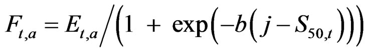
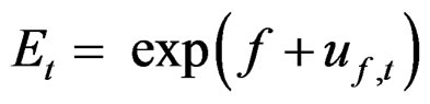
Catch at age data were simulated over 41 years (t = 1 – 41) starting of with a constant recruitment of 1 unit of fish (log recruitment r = 0) for the first years. There are 7 age classes (a = 3 – 9) in the data. The generated initial first year stock was balanced with respect to the input natural mortality (M = 0.2) plus fishing effort (E = 1, f = ln(E) = 0) with no error and a Logistic selection function of the age giving 50% selection at age 5 (S50 = 5) in the catch and with slope b = 0.7 at age S50. The fishing intensity is then 0.2E for the first recruited age class (a = 3) and 0.95E for the last (a = 9). There is no noise in the slope b, but year effects in the 50% selection age and in the log of the fishing effort  are both given by a first order auto-regressive process of the form:
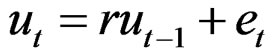
where  is iid N(0,
 ) and u0 = 0 for both:
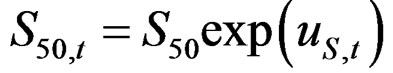
with , ln(
, ln( ) = –1.5 and ln(
 ) = –1. Additional noise in the fishing effort (d) is iid N(0,
 ) with ln(
 ) = –2. The selective fishing and total mortality by age and year is
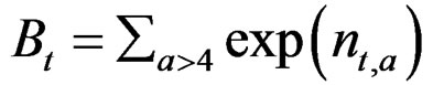
Zt,a = Ft,a + M The first two age classes are assumed not recruited to the fishery and invisible in the data so that the recruitment to age class 3 in year 4 is a Ricker function of the stock in year 1. The logarithm of the recruitment (r) for these first years was set 0. The spawning stock (B) was taken as the sum of the number of fish in age classes 5 - 9 in the data (thus knife-edge maturation 2 years after recruitment and no fish weights in the model)
The input parameters to the Ricker function are the logarithm of the spawning stock giving maximum recruitment: ln(Bmax) = –0.5, and the logarithm of maximum recruitment: ln(Rmax) = 0.4.

where  is iid N (0,
 ) with ln(
 ) = –0.5 The log of the stock is simulated with additional noise
where  is iid N (0,
 ) with ln(
 ) = –2.
This gives the log of the catch with observation error.
where is iid N (0, ) with ln(
 ) = –2.
No correlation structure was incorporated in the data generation or the models.
3. Estimation Procedure
The objective function (g) to be minimized is the sum of several terms each of which is summed over all appropriate t and a where they occur. For simplicity the summation symbols are left out here. Parameters 
 and all variances (
 ) are estimated back from the data.
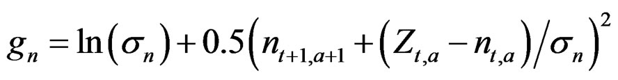
All models have the auto-regressive processes uS around S50 and uf around f that are state vectors (random effects) with the estimated variances  and
and  and the identical objective function components:
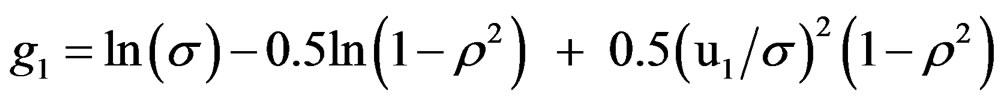
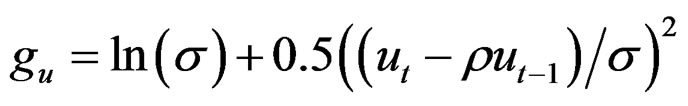
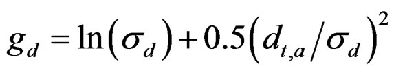
For the fishing effort the term guf is summed over all years, but for the selection pattern gus the first (same) value applies to the first 5 years and S50,t. is calculated as during the generation of the data. In the simpler models there is no error term dt,a estimated in the fishing effort so:
The log of predicted recruitment r is calculated as during the data generation and the variance  estimated:
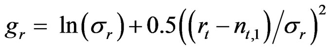
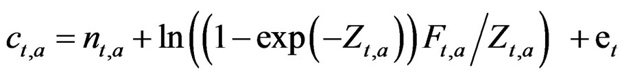
The catch is predicted as in the generation of the data and the observation error  is estimated from:
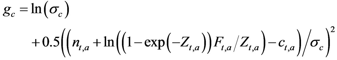
This objective function term differs in the models introduced later and additional terms occur in refined models below.
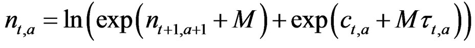
3.1. Base Model n – Z
The highest age stock (n∙,9) and stock in the final year (n41,∙) are both state variables (random effects). A temporary stock matrix n gets assigned these into the lower and left border values, and the stock back calculated deterministically using the fishing mortality as in conventional VPA [2]:
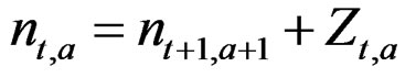 (1)
(1)
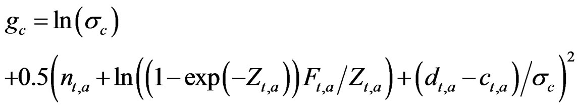
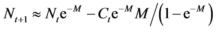
3.2. Base Model N – C
Here the stock is not updated using fishing mortality but with the catch added backward in time (VPA) so Equation (1) above is replaced by:
 (2)
(2)

In simulations  (see Appendix) can be calculated accurately (i.e. from the simulated true values, not the estimated values of F and Z) in order for the results of the two models to be exactly comparable in this respect. This equation will then give exactly the same results as (1) when the catch is according to the fishing mortality and there is no observation error. The catch is added to the stock at the end of the year (back calculated) rather than subtracting it from the stock at the beginning of the year, to avoid negative logarithms in the calculations.
The input variances for n and d do not occur as parameters in the above base models and are thus not estimated back. They can be seen as bounded to the value zero.
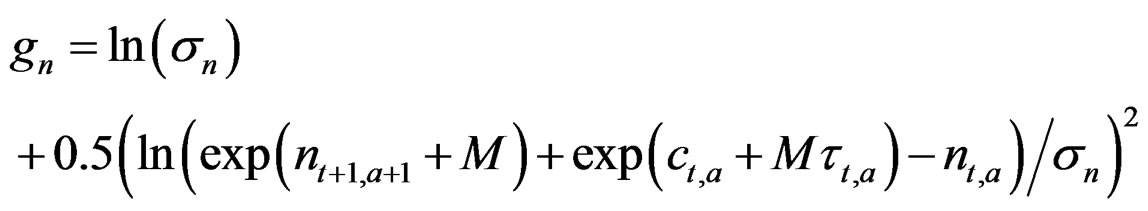
3.3. Refined Model n – Z*
Same as model n – Z above except that instead of just the highest age and last year stock, here the whole stock is a state space matrix. The stock therefore does not get calculated so Equation (1) is dropped, but a term is added to the objective function to link up the stock and estimate the variation, where the predicted stock is calculated as during the generation of the data:
The parameter  which includes variation in natural mortality (and migrations where plausible), is therefore estimated in this case, and in the models below. This was the model chosen to investigate the possibility of estimating M and what effect the size of the different input variances in the generated data had on its precision.
3.4. Refined Model N – C*
As N – C above except that as in the refined model above an objective function term replaces the stock Equation (2) and uses the catch to predict the stock change
3.5. Full Model n – Z**
Same as model n – Z* above with the addition of another state space matrix d (not including the last year and last age class). Now E (and F and Z) is calculated including d, and used in gc and gn.
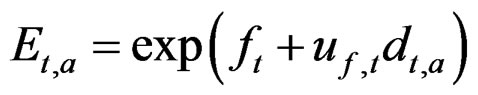
This is exactly as during the generation of the data. Thus d can here capture the fluctuations in the fishing intensity as it deviates from the separable E * S model. Accordingly a term to estimate its variance is added to the objective function:
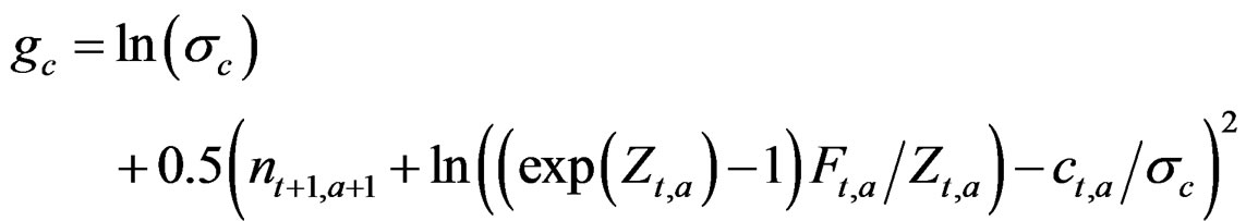
3.6. Full Model N – C**
Same as model N – C* above with the addition, as in the model n – Z** above, of a state space matrix d and the same term gd for its variance is added to the objective function. However d is not used in the calculation of F (which in this model is not used to update the stock) but rather d may correct for the observation error in the catch which would otherwise be propagated in the stock equation:
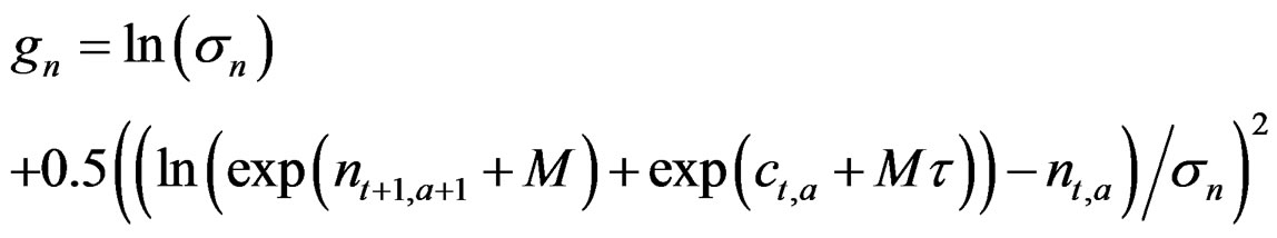
In fact the roles of  and
and  are in this case interchanged compared to their roles in the generation of the data so they would be expected to get estimated close to their respective values in the input reversed (the same value was used for both).
3.7. Models n + Z*, N + C, N + C* and N + C**
These models differ in that the predicted catch is related to the stock at the end of the fishing year so the fishing mortality gets estimated from:
A base n + Z model where the stock is updated deterministically using F is identical to the n – Z model, but due to the observation error in the catch not so when the stock is updated using the catch (N + C) nor in the refined models where there is noise in the stock equation (estimated  > 0).
> 0).
3.8. Penalized Maximum Likelihood Models
The base models n – Z and N – C were also estimated with penalized maximum likelihood (PL) where the state variables were treated as ordinary parameters to be estimated but penalized through the objective function terms gf and gs. One of the two AR(1) variances, either in the effort or in the selection always get lower bound with this method so the ratio of these variances was bound at the correct value and a single variance estimated. For additional comparison the terms gf and gs were dropped from the objective function and no auto-regression estimated (no penalty on yearly changes in effort and selection), referred to as UL.
3.9. Programming
All models used the same code to generate the data from the input parameters and the input seeds to the random number generator. The PL models were run in ADMB. The base IL models used exactly the same programs as the PL models but were run in ADMB-RE with the only change that the state variables were then declared as random_effects_vector. The estimation process starts with all parameters and state variables at their true values. Actually in ADMB-RE what is declared as random_effects can not be assigned initial values, so in fact all random_ effects were estimated as deviations from the simulated true values that are generated in the same program, but this is not presented as such here. The n – Z** model has both the whole stock n and the fishing mortality deviations d from the E*S model declared as a random_ effects_matrix. The n – Z* model uses the same program as n – Z**, but then d is fixed at zero. The base models n – Z and N – C where the stock is deterministically calculated were checked to give the same results as the n – Z* and N – C* models when the noise  in the stock relation term gn was bounded close to zero (but such runs take a much longer time than the simpler models). Bounds on all ln(
 ) were ±2 and on both ρ set 0.03 - 0.97. The program code is accessible online at http://www.hafro.is/ ~thg/langtn/re/cai/.
4. Results
For different methods and models Table 1 lists the input values used in generating the datasets and the estimates of corresponding parameters. Table 2 presents the percentage of runs where the estimates of the given parameters were lower bound. From the runs where the estimates were not lower bound the mean and the standard deviation around this mean was calculated and the mean of the Hessian estimated standard deviation as reported and its CV. The median of the parameter estimates is also given and the upper and lower 10 percentile.
The estimate of the final stock (in the last year) is of greatest interest to management. The deviations from the true values are known in these simulations so as a performance statistic the bias (mean log of the deviation) and the standard deviation of the estimated log of the final stock around the mean (coefficient of variation of the final stock) was chosen for presentation in Table 3 and the mean of the reported Hessian standard deviations of the log of the final stock as output (CV of final stock).
The base n – Z model with the IL method is relatively unbiased in all parameters except for a slight negative bias in the ρ in the AR(1) processes, in particular for the selection where also ρ is lower bound in 16% to 33% of the cases. There is a consistent negative bias in the log of the final stock of around –0.02 to –0.04 in the highest age, but compared to the realized CV of the results of around 0.25 this is negligible. Relating the fishing mortality to the stock at the end of the fishing year under the n – Z* model (that is n + Z*) gives almost identical performance,
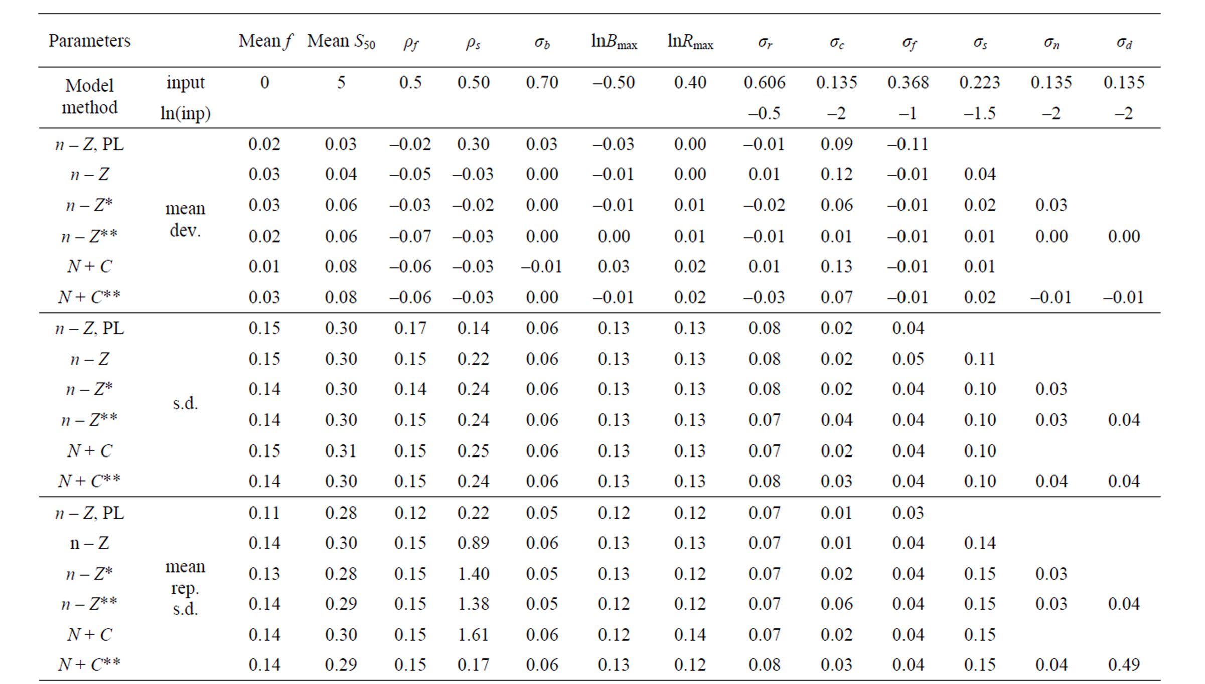
Table 1. Estimated parameters by different models. Method is integrated likelihood unless PL (Penalized Likelihood) is specified. Input values (log of the input variances also given). From datasets where not at lower bound: Mean deviation and standard deviation (from mean), mean reported standard deviation and CV. Median deviation and upper and lower 10% tile (for variances given in logarithms).
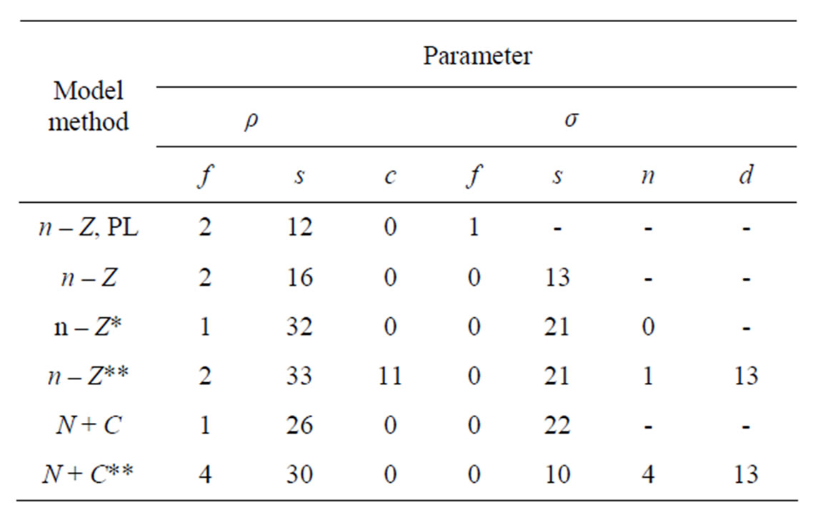
Table 2. Percentage of the 600 datasets (see Table 1) yielding lower bound estimates for parameters.
but is slightly more complicated so such results were not considered further.
With the Penalized Maximum Likelihood method the precision is poorer (in spite of the bound on the ratio of σs/σf at the correct value). In 1% of cases the estimate still gets lower bound. The ρ for selection is highly positively biased. The estimated precision of the final stock and variances is overestimated. Refinement in the models is not plausible with this method. With the IL method the precision improves (realized CV decreases) with more refinement in the models (n – Z* and n – Z**). Variances then get increasingly estimated at the lower bound and their precision is then underestimated on average. On inspection precision is estimated too poor when variances are estimated too small, but overestimated for high values. The highest estimates deviate significantly from the true value based on the reported precision.
In the base n – Z and N – C models the reference case always gets a nonzero estimate of the yearly variation in f but the yearly variation in S50 is bound at the lower limit in some cases. Other variances that are included in these base models do get nonzero estimates most of the time and the internal variation is mostly reflected in a higher estimate of σc. In the full models all parameters and variances are estimated back. In the n – Z** model all variances are relatively unbiased (estimates at the lower bound not included) and the reported precision is in good agreement with the realized mean precision. The estimates of the variances σc and σd are inversely correlated and never both lower bound.
When the stock was updated with the Pope approximation by subtracting the catch at the middle of the fishing year (τ = 0.5) the precision is similar to other methods but the final stock is positively biased by around 0.25. If τ is calculated accurately from the simulated true values of F and Z and results differ only in the fourth significant digit to those obtained with τ calculated from the estimated values. The N – C model then has a negative bias in the final stock that increases with age (8% - 17%).
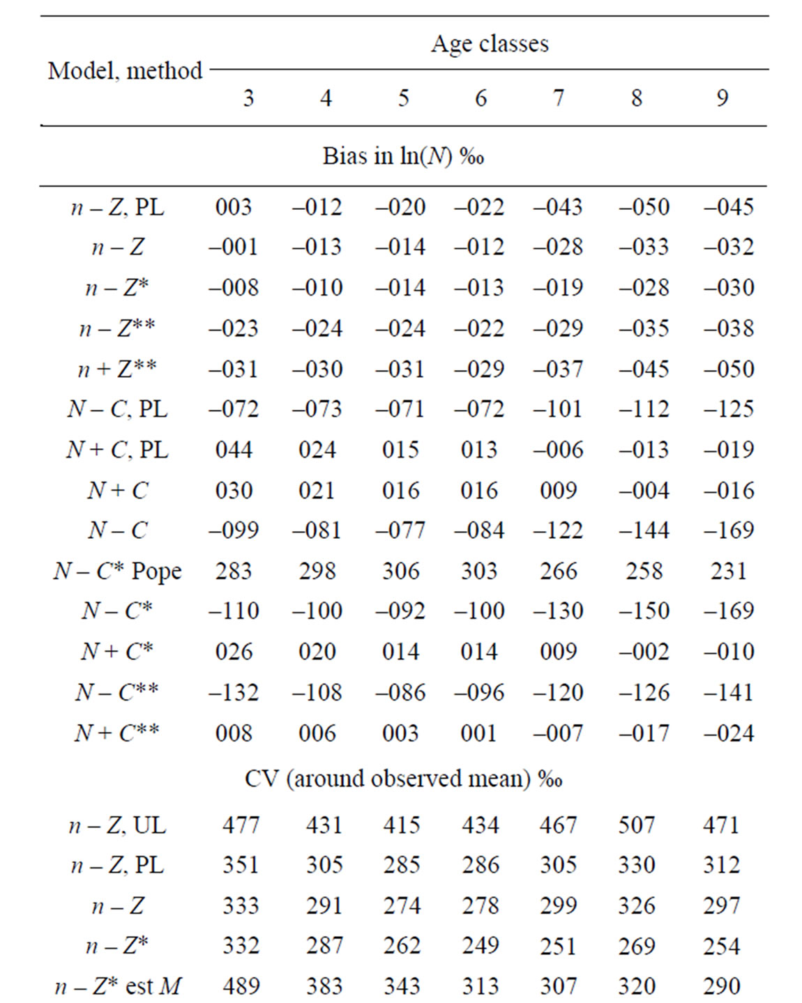
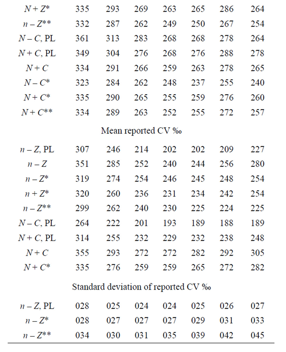
Table 3. Final stock precision. Method is integrated likelihood except for lines marked UL (unconstrained effort) or PL (Penalized Likelihood). Same 600 datasets as in Table 1.
The bias is somewhat less in the refined N – C** model where the observation error in the catch is estimated and accounted for. In the N + C models where the fishing mortality (F) is related to the stock at the end of the fishing year, the bias is only to the same small degree as in the n – Z models. The PL method has better precision with the N + C than n – Z model.
Table 4 shows the sensitivity of the precision in the final stock to the input variation in the simulated data. Changes in the σ for recruitment are mostly reflected in the precision in the first ages, but the reverse is true for the observation error in catch and the deviations from the E * S model.
The estimate of M (natural mortality) obtained from the n – Z model with the PL method and the IL method with model refinements is given in Table 5. The precision in M is extremely poor with the reference case used above so the reference case for studying M was chosen with lower variation in both the recruitment (r) ln(σ) = –1 and selection (s) ln(σ) = –2, but higher in the effort by year  ln(σ) = –0.5. The estimate of M obtained with the PL method is rather meaningless due to the high variation and negative bias. The IL method is only slightly biased in the base n – Z model, and the refined models are less biased and provide additional 9% improvement in the accuracy in M.
The sensitivity in the estimate of M and its precision in model n – Z*, obtained by varying the size of the differrent input variances in the generated data is shown in Table 6. Solving for M is singular when there is no between years variation in fishing effort and accordingly the precision in M improves as σ for f increases. When other variation is small an increase is reflected up to 100% in better precision in M, but for very high variation the precision degrades again. Conversely, an increase in all other variation degrades the precision in M, as expected. The biggest impact is from σ for r where a change over a wide range is reflected 45% in the precision in M. The deviations in recruitment affect a cohort at all ages whereas the variances for n or d affect a single year-age group. A change in σ for either of these is reflected by a 15% - 18% change in the precision in M, but for selection (s) the change is only about 4%. This variation was put only on the age at 50% recruitment and not in the slope of the selection function (b), which is more highly correlated with the estimate of M. Estimating M severely reduces the precision in the final stock, in particular in the first age groups shown in Table 3 and doubles the standard deviation of its reported CV.
5. Discussion
Ignoring the auto-correlation over time in the fishing mortality can lead to very poor precision in the final stock
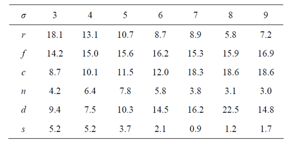
Table 4. Sensitivity in observed CV in final stock to input variation increase to ln(σ) + 0.5. Reference case n – Z* model in Table 1, 300 datasets.
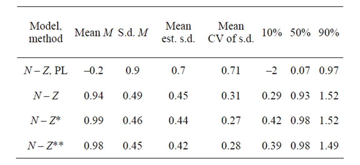
Table 5. Estimates of M given as proportion of the input value 0.2 by different methods and models. Reference case σf higher and σr and σs lower by 0.5 than in reference case runs above, 600 datasets.
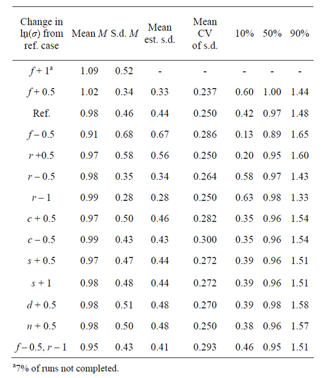
Table 6. Sensitivity of the estimate of M to the input variances. Model n – Z*, IL, 300 datasets. Reference case as in Table 4.
(given in Table 3 line marked UL). The base model with the PL method and the ratio of the variances in f and s fixed at the correct value does not differ greatly from the IL method. There is considerable bias in ρs and slightly poorer precision in parameters and the final stock by about 2%. The output CV of the final stock is also underestimated. The improvement in precision in the final stock comes with the estimation of the internal variances σn and σd that is only possible with the IL method. Testing of other additional parameters with the PL method may be meaningless as seen from the estimation of M. In real datasets the variance of the catch observation error generally differs by age (higher for older/youngest age groups). With the IL method a random walk by age or variation from a common mean can be tested and is rejected (associated variance estimated zero) in all 300 datasets (and so at no cost). An independent variance can also be estimated for each age at a cost of slightly reduced precision. With the PL method, however, the variance for one age will generally tend to zero with infinite likelihood, so some functional form by age and other constraints are needed in order to get reasonable results, but the outcome may then depend on what assumptions are made.
Using the Pope approximation has little effect on the precision. The approximation is close at the lowest age but the subtracted catch at the highest age is about 2% too much. This slight skewing of the selection function leads to a 25% positive bias in the final stock in Table 3. The exact N – C model turned out to be rather negatively biased. As the observation error in the catch is log-normal the total subtracted catch is too large by exp (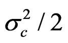 ) and an attempt was made to correct for this by dividing the catch by this factor in the stock equation, but with no success. The stock is in effect back calculated to avoid drifting into logarithms of negative numbers. To balance this asymmetry the fishing mortality F was related to the stock at the end of the year in the catch equation. This had little effect in the n – Z model but slightly poorer precision. The bias in the N – C model was eliminated and this model is referred to as N + C. With this model there is less difference between the PL and IL methods and between the N + C and N + C** model which has almost as good precision as the n – Z** model (1% poorer).
The N – C models get the changes in the stock better in line with the actual catches, which may make for a more appealing presentation. Another approach to this has been suggested (D. Fournier pers. comm.) where the predicted catch is derived from the change in the stock, so gc minimizes the square of:
This caused computational problems (the difference drifts to zero) in several datasets. This could be sidestepped, but then produced an implausible stock in 10% - 15% of the datasets and surprisingly resulted in a non-positive Hessian in another 10% of cases, so a full comparison could not be made, but bias and precision appeared to deteriorate slightly.
Survey series with constant (or known) effort and standardized methods and gear have been conducted around Iceland, but survey effort is low compared to fishing effort and variation in effort and selection pattern is larger than in the catch data. The relationship of the survey index to stock size may be nonlinear. For these reasons no survey data were simulated in this exercise as the assumptions that need be made are case specific and will largely determine the outcome. However, surveys provide indices of the stock also at young ages that are not, or poorly observed in the catch and therefore in particular reduce the uncertainty in the final stock at young age and prognosis. M may be pinned down with assumptions about the constancy by age, or functional form of the survey selection pattern, but the reduced uncertainty in year class strengths that may result from inclusion of surveys would in particular better the precision in the estimate of M.
The estimates of M. and F are highly negatively correlated. Relative changes in F over time are penalized in the model and these changes can be made relatively smaller with a lower estimate of M and higher values of F. This is what causes the negative bias in the estimate of M. If M is to be estimated the changes in log(Z) should be penalized rather than the changes in f, to avoid this bias. This involves changing a single line of code.
6. Conclusions
In this simple example the PL method given the prior input needed for it to work is outperformed by the IL method. In more realistic examples the PL method requires still more prior input. Estimation of M is not plausible with the PL method. Post-war variation in fishing effort has been low and management objectives aim at constant fishing mortality, while the noise in recruitment is high for the main commercially exploited species off Iceland, so the prospects of estimating M are poor even with the IL method. Aanes et al. [10] came to a similar conclusion. The IL method allows for estimation of internal unobserved variation that improves the precision. Such models should be tested, although zero estimates of some component of the variation is common (absorbed by a different component) and the true variation may be significantly less than implied by the reported precision. The estimation of the internal unobserved variation likely reduces correlation in residuals that may then be ignored. However, estimation of a correlation structure is not problematic with the IL method, although computationally more intensive. Updating the stock with the catch (N − C or better N + C for less bias) seems to be more robust in simple models but more complex and in the full model slightly outperformed by the more common method of using the estimated fishing mortality to update the stock (n − Z), with the level of variation tested here. Looking at results from both approaches might be worth while.
7. Acknowledgements
This work was inspired by Gudmundur Gudmundsson, Science Institute, University of Iceland. Thanks to David Fournier admb-project.org for enlightening comments.
REFERENCES
- J. G. Pope, “An Investigation of the Accuracy of Virtual Population Analysis,” International Commission for the Northwest Atlantic Fisheries Research Bulletin, Vol. 9, 1972, pp. 65-74.
- A. D. MacCall, “Virtual Population Analysis (VPA) Equations for Nonhomogeneous Populations, and a Family of Approximations Including Improvements on Pope’s Cohort Analysis,” Canadian Journal of Fisheries and Aquatic Sciences, Vol. 43, No. 12, 1986, pp. 2406-2409. doi:10.1139/f86-298
- T. A. Branch, “Differences in Predicted Catch Composition between Two Widely Used Catch Equation Formulations,” Canadian Journal of Fisheries and Aquatic Sciences, Vol. 66, No. 1, 2009, pp. 126-131. doi:10.1139/F08-196
- A. C. Harvey, “Forecasting Structural Time Series Models and the Kalman Filter,” Cambridge University Press, Cambridge, 1989.
- G. Guðmundsson, “Time Series Analysis of Catch-at-Age Observations,” Applied Statistics, Vol. 43, No. 1, 1994, pp. 117-126. doi:10.1016/0167-6687(94)90696-3
- P. de Valpine and R. Hilborn, “State-Space Likelihoods for Nonlinear Fisheries Time-Series,” Canadian Journal of Fisheries and Aquatic Sciences, Vol. 62, No. 9, 2005, pp. 1937-1952.
- H. J. Skaug, “Automatic Differentiation to Facilitate Maximum Likelihood Estimation in Nonlinear Random Effects Models,” Journal of Computational and Graphical Statistics, Vol. 11, No. 2, 2002, pp. 458-470. doi:10.1198/106186002760180617
- H. J. Skaug and D. A. Fournier, “Automatic Approximation of the Marginal Likelihood in Non-Gaussian Hierarchical Models,” Computational Statistics & Data Analysis, Vol. 51, No. 2, 2006, pp. 699-709. doi:10.1016/j.csda.2006.03.005
- ICES, NWWG Report, 2011. http://www.ices.dk/reports/ACOM/2011/NWWG/Sec10Icelandichaddock.pdf
- S. Aanes, S. Engen, B. Sæther and R. Aanes, “Estimation of the Parameters of Fish Stock Dynamics from Catch-atAge Data and Indices of Abundance: Can Natural and Fishing Mortality Be Separated?” Canadian Journal of Fisheries and Aquatic Sciences, Vol. 64, No. 8, 2007, pp. 1130-1142. doi:10.1139/f07-074
Appendix
With natural mortality M and continuous harvesting with fishing mortality F. Denote total mortality Z = M + F. The stock at start of season t + 1 is calculated as:
 (1)
(1)
 (2)
(2)
Can be approximated by removing all the catch at a time  of the season t:
 (3)
(3)
and will be exact when  is:
is:
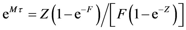 (4)
(4)
A first order approximation [1] is:
 ≈ 1/2 (midseason) which is too large (late) for all F + M > 0.
A second order approximation:

is much closer, but too small (early) for large values (by >0.01 when Z + F > 3).
MacCall [2] improved on Pope’s approximation by setting F = 0 in the second equation:
As seen from the second order approximation the effect of F is double that of M, and F is in many practical cases larger than M so in general this improvement is small. If the purpose is to eliminate F, then the exact form in Equation (2) or (3) (or the second order approximation) with a reasonable constant value for F by age/season should rather be used.