ABSTRACT

Genetic effect estimates for loci detected in quantitative trait locus (QTL) mapping experiments depend upon two factors. First, they are parameterizations of the genotypic values determined by the model of genetic effects. Second, they are consequently also affected by the regression method used to estimate the genotypic values from the observed marker genotypes and phenotypes. There are two common causes for marker-genotype data to be incomplete in those experiments—missing marker-genotypes and within interval mapping. Different regression methods tend to differ in how this missing information is represented and handled. In this communication we explain why the estimates of genetic effects of QTL obtained using standard regression methods are not coherent with the model of genetic effects and indeed show intrinsic inconsistencies when there is incomplete genotype information. We then describe the interval mapping by imputations (IMI) regression method and prove that it overcomes those problems. A numerical example is used to illustrate the use of IMI and the consequences of using current methods of choice. IMI enables researchers to obtain estimates of genetic effects that are coherent with the model of genetic effects used, despite incomplete genotype information. Furthermore, because IMI allows orthogonal estimation of genetic effects, it shows potential performance advantages for being implemented in QTL mapping tools.

1. INTRODUCTION

Quantitative trait locus (QTL) mapping experiments aim to detect loci that significantly contribute to the variance of a phenotype in a particular population [1]. In these experiments, models of genetic effects, also called genotype-to-phenotype maps [2], enable researchers to evaluate the effects of allele substitutions in positions across the genome. In QTL mapping, these models are thus used in a reverse manner, starting from the phenotypes to obtain the genetic effects of genotypes in the evaluated loci. After the QTL are mapped their effects are usually provided using the particular model parameterization that was chosen for mapping them. We refer to these initial estimates as the raw estimates that come as a direct result of the QTL mapping experiment.  

The use of additional genetic models makes it possible to reparameterize the raw estimates so that they are adequate for addressing different topics of evolutionary interest (see e.g. [3-7]). We note, though, that this way of assigning a meaning to the genetic effects relies on whether the raw estimates actually match the model of genetic effects used to obtain them, or not. Therefore, besides choosing an appropriate model of genetic effects, it is also necessary to make sure that, in practice, the regression method used provides estimates matching that model.

Missing genotype information has routinely been pervasive in QTL analysis for two main reasons. First, molecular methods for marker genotyping have been prone to wrong and failed detection, leading to a non-negligible percentage of missing marker genotypes in the datasets. Second, genotypes are missing and thus have to be inferred when inspecting loci within marker intervals, i.e. when performing interval mapping (IM) [8-10]. In this communication we elaborate on how missing genotype information—regardless of its cause—distorts the estimates of genetic effects obtained in QTL mapping experiments when a standard regression method is used. We then propose an alternative regression method that avoids this source of bias—i.e. it provides estimates of genetic effects that are coherent with the model of genetic effects used, even with missing genotype information. We illustrate the advantages of this method using a numerical example and point out some convenient properties for its potential use in QTL mapping applications.

2. REGRESSION-BASED ESTIMATION OF GENETIC EFFECTS

In a QTL mapping experiment, genetic effects of loci can be estimated from observed genotypes and phenotypes of individuals using the regression:

, (1)

where is the vector of observed phenotypes, X is the regression design matrix, E is the vector of genetic effects and ε is the vector of residuals. For performing the regression, a choice for the regression design matrix needs to be done. This matrix can be decomposed into two matrices:

, (2)

where the incidence matrix, Z, entails a genotype probability vector for each phenotype observation. Z can be used to map genotype effects into individual estimates:

. (3)

Hence, the incidence matrix Z determines how the genotypic values are estimated from the data.

The matrix S in (2) is called the genetic-effect design matrix and it is built to reparameterize the genotypic values into genetic effects [11]:

. (4)

This expression entails a decomposition of the genotypic values, G = (G_ij), into additive (average allele substitution) effects (α_i) and dominance deviations (δ_ij) from a reference point (µ), G_ij = µ + α_i + α_j +δ_ij, (for details see [3]). In other words, S is the model of genetic effects that determines how the genetic effects, E, are defined in terms of the genotypic values, G. Note that the regression-based estimation of genetic effects (1) can be recovered by combining expressions (2-4).

The IM method [8] set a landmark in the estimation of genetic effects. Using interval mapping it became possible to obtain both estimates of genetic effects within marker intervals and to more efficiently analyze data with missing marker genotypes. However, the original IM was based on a computationally demanding maximum-likelihood estimation procedure. Therefore, linearregression methods enabling faster estimation of genetic effects with missing data were developed [9,10]. These methods are still convenient, especially when addressing searches in massive datasets, e.g. microarray expression QTL (eQTL), QTL mapping of epistasis and permutation testing with many iterations. Hereafter we show that a common method of choice, the Haley-Knott regression (HKR) method, can be described in terms of the matrices Z and S introduced above (3, 4).

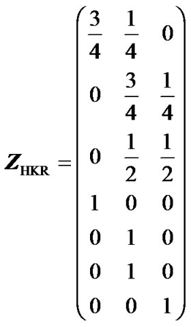
HKR is based on the computation of genotype probabilities for all m possible genotypes of a locus, for the n individuals sampled [9,10]. The estimation of genetic effects is conducted through a regression of the phenoltype on these genotype probabilities. Each set of m genotype probabilities for each individual enter the regression as a row in the n × m Z-matrix (3). For instance, the HKR Z-matrix for a one-locus two-allele case is:

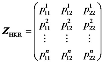, (5)

where denotes the probability that individual k has genotype ij.

The genetic model used in the original HKR is Fisher’s [12] population-independent parameterization, called the F_∞ model [13]. Thus, the S-matrix of HKR is the matrix S_F∞ [3,14]. However, it has frequently been suggested that estimates of genetic effects should instead be obtained using models that are orthogonal for the (specific samples of) populations under study [3,14-16]. That individual effect estimates remain unaltered in reduced models is one of the convenient outcomes of orthogonal estimation of genetic effects. As an example, orthogonal estimates of genetic effects for an ideal F₂ population can be obtained using Fisher’s [12] F₂ model with genotype frequencies (p_ij) = (1/4, 1/2, 1/4). The genetic-effect design matrix of this model is:

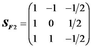. (6)

Similar expressions for more general cases than the particular F₂ population have been provided, accounting for alleles with different frequencies [14] and for departures from the Hardy-Weinberg proportions [3].

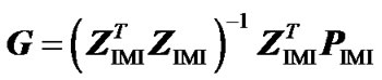
When assessing whether the estimates of genetic effects coming from (1) are orthogonal for a particular population, complete genotype information is often assumed. However, Álvarez-Castro and Carlborg [3] have shown that obtaining orthogonal estimates of genetic effects also relies on incidence matrices fulfilling the condition:

, (7)

where the operator Diag generates a diagonal matrix from a vector and T gives the transpose matrix. This desirable condition is achieved with incidence matrices having one only non-zero value per row, which does not hold for Z_HKR (5) with incomplete genotype information. Indeed, Z_HKR (5) does not in general, when combined with (3), lead to genotypic values that are means of the observations, as shown below using a counter-example. It is thus not surprising that such estimates of genotypic values distort the properties of the genetic effects in (1)—that are given by the genotypic values and the genetic-effects design matrix through (4)—whether those properties are related to orthogonality or not. In the following section we propose an alternative way of performing regression (1) that can be used to overcome these problems.

3. INTERVAL MAPPING BY IMPUTATIONS, IMI

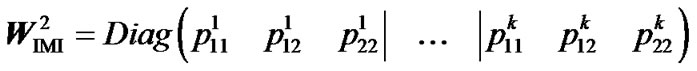
Here we describe how to build a regression method that fulfils condition (7) and leads to genotypic values that are weighted means of the data. We do this by following a strategy of multiple imputed genotype realizations of the individuals in the population [17,18]. We split the representation of each individual in Z_HKR (5) into as many imputations as there are possible genotypes, m. In its turn, we then weight each imputation by the square roots of the m genotype frequencies of the n individuals of the sample. In mathematical terms, we multiply a diagonal matrix containing the square roots of all genotype probabilities, W_IMI, to a column of n identity matrices of dimension m, I_IMI:

. (8)

We have added horizontal lines to mark the separate blocks representing each of the individuals.

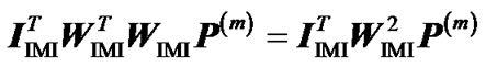
Using the above matrix (8), we present the interval mapping by imputations (IMI) regression-based method for estimation of genetic effects as using the nm ´ m incidence matrix Z_IMI (8) within Equation (1) under a weighted-regression framework. It is worth to mention here two particular features of this framework (for further details see e.g. [19]). First, the vector of phenotypic observations, P (1, 3), has to be weighted in accordance with Z_IMI as P_IMI = W_IMIP^(m), where P^(m) is the vector in which each element of P occurs m times. Second, the matrix W_IMI (8) reveals that we are using the Haley-Knott genotype probabilities—, cf. (5)—as weights (note that the matrix of weights is implemented with the square roots of the weights instead of with the weights themselves). When using IMI through (1), the S-matrix (2, 4) can be chosen to fit the population under study for X^TX to be diagonal whenever Z^TZ is. In particular, the S-matrix shall accommodate the frequencies at the diagonal of (Z^TZ)/n [3].

4. DEMONSTRATION OF THE MAIN PROPERTIES OF IMI

We have postulated IMI to fulfil two major properties. These are condition (7) and providing weighted means of observation through regression (3). First, taking into account that matrix (8) has one only non-zero value per row, it is easy to see that it fulfils condition (7).

Second, to check that Z_IMI (8) provides genotypic values that are means of the observed data points, weighted by their certainty, we consider it within the normal equation of regression (3) as, leading to:

. (9)

Now we compute separately the two terms at the right hand side of this equation. We first get

Then, using that:

,(10)

we obtain

hence:

.(11)

Next we expand the second term as =. From this, using (10) again, we obtain:

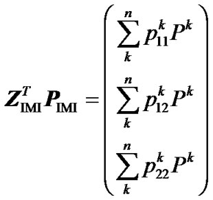. (12)

Finally, from (9, 11, 12) we get the genotypic values as the vector

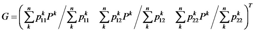whose scalars are the means of the observed phenotypes of each genotype, weighted by the certainty of the assignments between the phenotypes and the genotypes, QED.

5. NUMERICAL EXAMPLE

Here, we illustrate the use and the advantages of IMI through a very simple example. First, we show how missing genotype information distorts the estimates of genetic effects when using the Z-matrix in expression (5) and then we show that these problems fade away when using IMI. The genotype data in this example is a small sample population of seven individuals genotyped for one locus with two alleles, A₁ and A₂. There is incomeplete information for individuals 1, 2 and 3—individual 1 could be either A₁A₁ or A₁A₂ with probabilities 3/4 and 1/4, individual 2 could either be A₁A₂ or A₂A₂, with probabilities 3/4 and 1/4, and individual 3 could be A₁A₂ or A₂A₂, with equal probabilities. The genotype is known for individuals 4 to 7, which have genotypes A₁A₁, A₁A₂, A₁A₂ and A₂A₂, respectively. Thus, the HKR Z-matrix (5) for this case is:

. (13)

Note that the first three rows contain multiple nonzero elements, reflecting the missing genotype information of individuals 1 to 3. The column averages of matrix (13) are 1/4, 1/2 and 1/4—this population does therefore have the properties of an ideal F₂ population, whose genetic-effect design matrix, which should give orthogonal estimates of the genetic effects, is given in expression (6). The HKR X-matrix, X_HKR, can then be computed using expressions (2, 6, 13). If our case was not an ideal F₂ population, a different matrix than (6) would be used to account for its genotype frequencies [3].

The phenotype data is given in the following vector of phenotype observations:

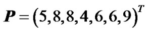. (14)

We now have all required components to use expression (1) for performing a regression-based estimation of genetic effects. We have actually used three different variants of matrix (6). The first one is the complete matrix (6), corresponding to the full model including both additive and dominant effects as deviations from the population mean, G_ij = µ + α_i + α_j + δ_ij. Secondly, we have considered a purely-additive reduced model assuming no dominance interaction, G_ij = µ + α_i + α_j, by setting the last column of matrix (6) to zeros. Lastly, we have considered a purely-dominance reduced model where the additive effects are assumed to be zero, G_ij = µ + δ_ij, by setting the second column of (6) to zeros. These two reduced models represent two complementary components of the full model given by (6).

By implementing these models to perform HKR using the data above we have obtained two main noteworthy results (left-hand side of Table 1). First, the genotype value estimated using HKR for the genotype “22”, G₂₂ = 9.30, lies outside the range of the phenotype observations in vector P (14) (see Figure 1). This result does not depend upon which genetic-effect design matrix—i.e. the S-matrices of the full or of the reduced models—we are implementing in regression (1). Its cause is instead that the incidence matrix—i.e. the Z-matrix in (2)—connects the observations (14) and the genotype values in a nonoptimal way.

Second, using expression (3) we can demonstrate that these inconsistencies in the genotypic values are distorting the estimates of genetic effects. Indeed, although we have chosen a model of genetic effects (6) in accordance with our genotype data for providing orthogonal estimates of genetic effects, Table 1 shows that in practice the resulting estimates are not orthogonal. For instance, the estimate of the additive effect of the purely-additive model is different from the estimate of the additive effect in the full model when using the Z_HKR matrix (13). This distortion of the genetic effects becomes stronger for the purely-dominance model, where the dominance estimate is of opposite sign to the estimate obtained using the full model. More to the point, the variances associated with the estimates behave in the same way—the explained variance () of the full model is not the sum of the explained variances of the two complementary reduced models (), which would be the case if the estimates were orthogonal.

This lack of orthogonality of the estimates can also be tested beforehand, by computing the matrix-product of the X-matrix and its transpose, which is diagonal if and only if the X-matrix leads to an orthogonal estimation of genetic effects (for details see [3]). That product is:

, (15)

which is not diagonal. This fact is in agreement with the observations of Álvarez-Castro and Carlborg [3], who have shown that obtaining orthogonal estimates of genetic effects relies on incidence matrices fulfilling the condition (7), as mentioned above.

Hereafter, we show that IMI provides genotypic values as weighted means of the observations and orthogonal estimates of genetic effects when using a geneticeffect design matrix that is orthogonal for the population under study. The incidence matrix of IMI (8) for this example is:

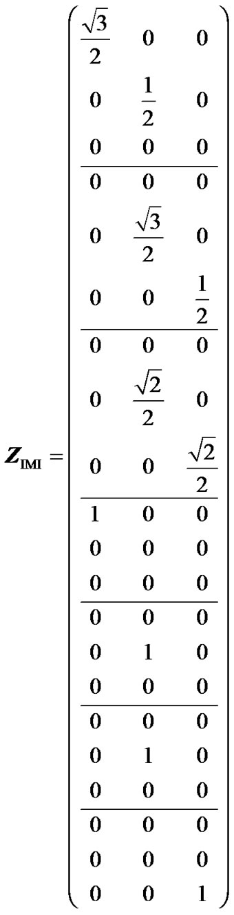(16)

Because this matrix has one only non-zero value per row, it fulfils (7) and it therefore enables us to perform orthogonal estimates of genetic effects. We can doublecheck this by computing X_IMI, through (2, 6, 16), analogously to how we obtained X_HKR (15) above:

.

This is a diagonal matrix, which implies that the estimates obtained when implementing X_IMI in regression (1) are orthogonal. Indeed, all the estimates obtained using IMI for the data of the numerical example above (right hand side of Table 1) remain unaltered when reducing the full model to both the purely-additive and the purely-  dominance models. Note also that the explained variances of these two complementary reduced models sum up to the explained variance of the full model. The inconsistencies we noted above regarding the genotypic values obtained using Z_HKR (13) have also vanished when using Z_IMI (16) instead. In particular, each genotypic value associated to IMI is the weighted (by the genotype probabilities) mean of the phenotypes of all individuals possibly having that genotype (see Figure 1), as proved analytically above (9-12). This is in accordance with the case of no missing information. Altogether, we have verified that IMI enables us to obtain estimates of genetic effects that are coherent with whichever model of genetic effects we would like to implement—in our example, the F₂ model (6) orthogonally fitting the data—despite missing genotype information.

6. DISCUSSION

The IMI method uses an imputation-regression approach for computing estimates of genetic effects of e.g. loci detected in a QTL mapping experiment. We have shown that a key difference between IMI and HKR is that the latter implements the genotype probabilities into an incidence matrix (5) with multiple non-zero values per row. IMI uses the Haley-Knott genotype probabilities [9,20] in a different way, better handling uncertainty and consequently leading to estimates of genetic effects that are coherent with the model (i.e. the S-matrix) implemented to obtain them.

Throughout this communication we have presented and elaborated on the IMI regression method and compared some properties of this method with the HKR, which is a standard, landmark method used for estimation of genetic effects in QTL mapping experiments. Other regression methods have been developed to obtain estimates of genetic effects. For instance, the estimating equation (EE) method [21] has been developed to reduce a bias found to occur in the residual variances provided by HKR [22], with the drawback of higher computational requirements. Similar to HKR, the EE method (or any other method to the best of our knowledge) does not provide estimates of genetic effects that are coherent with the genetic model used, in particular with respect to providing orthogonal estimates when using orthogonal models of genetic effects. It is noteworthy that IMI provides estimates that are coherent with the choice of both the model of genetic effects and also with the weights assigned to the uncertain observed genotypes. In our demonstration, we have assumed these weights to simply be the genotype probabilities. Other weighting choices are also possible. Whatever the chosen weights, our demonstration would still hold—the estimated genotypic values are always the means of the observed genotypic values, weighted in the way given by the scalars in vector W_IMI.

The main reason to be aware of the meaning of the raw estimates of genetic effects as they come from a QTL mapping experiment is not that we will necessarily be interested in drawing specific conclusions directly from them. Models of genetic effects exist that are associated to different meanings of evolutionary interest, from effects of allele substitutions in particular genetic backgrounds to average effects of substitutions at the population level where polymorphism exist at multiple loci (see e.g. [23]). Conveniently, it is feasible to translate the genetic effects obtained using one model to those of another model when the original underlying parameterization (S-matrix) is known [3,24]. It is therefore not necessary to implement a QTL mapping tool with the particular S-matrix that will provide the set of estimates that is needed to address a particular problem (in fact, several S-matrices and sets of estimates will be involved when the same data is to be used for multiple purposes). What is needed instead is an estimation method that guarantees that the initial set of estimates of effects obtained in a QTL mapping experiment fits in a coherent manner to a parameterization (whichever one), from which it is then possible to obtain the genetic effect estimates needed for addressing any particular question. We have shown that IMI guarantees such coherent estimates and is therefore the most appropriate method to use for obtaining estimates of detected QTL. These estimates should then be reported instead of the raw estimates coming from whatever regression method was used to map the QTL. By reporting IMI estimates of QTL together with information on the model of genetic effects used to obtain them, researchers of original communications would provide valuable information to other scientists that wish to e.g. compare results from different studies.

Moreover, IMI is a convenient method to be implemented in a QTL mapping tool. Models of genetic effects exist that are orthogonal for populations other than the F₂ that we used in our example [3,14,16]. Since IMI can be used to provide orthogonal estimates of genetic effects, it may highly facilitate model selection strategies—i.e. finding the statistically optimal genetic architecture fitting the data. The IM [8] and the HKR [9] are known to bias upwards the odds of QTL at low-information-content regions (e.g. generating concave arches of the LOD-score functions inside marker intervals). This can be addressed with IMI, which provides a better management of uncertainty leading to the computation of more appropriate residual variances. In that respect, it makes sense to further refine the vector of weights of IMI so that it accounts for the particular information content at each individual position tested. Once a choice for these weights is made, a model of genetic effects fitting the frequencies (p_ij) such that Z^TZ = nDiag(p_ij) shall be used [3]. A major motivation for tuning the implementation of IMI for QTL mapping is that orthogonal estimation of parameters is computationally very efficient as compared to traditional linear regression methods (Harling, Nettelblad and Holmgren, in preparation). However, a detailed implementation of IMI for mapping QTL is out of the scope of this communication.

Lastly, we are aware that in the light of the latest and ongoing progress in experimental techniques—in particular the advent of increasingly dense marker maps based on single-nucleotide polymorphisms (SNPs)—it could be perceived that the concept of IM is becoming obsolete. We concur that this could be the case for some types of pedigrees, for which highly informative local marker windows (or single markers) can enable conclusive allele-origin determination. However, if the founder individuals share a relatively recent common ancestor (e.g. due to artificial breeding or population bottlenecks), SNP maps intended for the species at large might fail to accurately identify polymorphic regions. As an example, a stretch of 10 s of cM in length can lack the needed data to make a conclusive discrimination of alleles since it is possible that the genetic polymorphisms underlying the phenotypic variation are more recent than the SNPs used for mapping. It is well-known for instance that short tandem repeats frequently display a mutation rate that is multiple orders of magnitude higher than that of SNPs [25], and several quantitative traits have been linked directly to repeat-count variability. These are examples in which an interval mapping approach—where the allele origin is assessed based on a model of recombination and the closest linked markers with discriminating power— keeps on performing better than simpler window-based trait association methods.

7. ACKNOWLEDGEMENTS

CN was funded by The Graduate School in Mathematics and Computing (FMB), Sweden. ÖC was funded by a EURYI Award and a Future Research Leaders grant from SSF. JÁC was funded by an “Isidro Parga Pondal” contract from the autonomous administration Xunta de Galicia and by research projects BFU2009-11988 and BFU2010-20003 form the Spanish Ministry of Science and Innovation. The authors thank Ricardo Pong-Wong for fruitful discussion.

REFERENCES

- Wu, R., Ma C.-X. and Casella, G.C. (2007) Statistical genetics of quantitative traits: Linkage, maps and QTL. In: Gail, M. et al. Eds. Statistics for Biology and Health, Springer, New York.
- Lewontin, R.C. (1974) The genetic basis of evolutionary change. Columbia University Press, New York.
- Álvarez-Castro, J.M. and Carlborg, Ö. (2007) A unified model for functional and statistical epistasis and its application in quantitative trait loci analysis. Genetics, 176, 1151-1167. doi:10.1534/genetics.106.067348
- Álvarez-Castro, J.M., Le Rouzic, A. and Carlborg, Ö. (2008) How to perform meaningful estimates of genetic effects. PLoS Genetics, 4, e1000062. doi:10.1371/journal.pgen.1000062
- Besnier, F., Le Rouzic, A. and Álvarez-Castro, J.M. (2010) Applying QTL analysis to conservation genetics. Conservation Genetics, 11, 399-408. doi:10.1007/s10592-009-0036-5
- Le Rouzic, A. andÁlvarez-Castro, J.M. (2008) Estimation of genetic effects and genotype-phenotype maps. Evolutionary Bioinformatics, 4, 225-235.
- Le Rouzic, A., Álvarez-Castro, J.M. and Carlborg, Ö. (2008) Dissection of the genetic architecture of body weight in chicken reveals the impact of epistasis on domestication traits. Genetics, 179, 1591-1599. doi:10.1534/genetics.108.089300
- Lander, E.S. and Botstein, D. (1989) Mapping mendelian factors underlying quantitative traits using RFLP linkage maps. Genetics, 121, 185-199.
- Haley, C.S. and Knott, S.A. (1992) A simple regression method for mapping quantitative trait loci in line crosses using flanking markers. Heredity, 69, 315-324. doi:10.1038/hdy.1992.131
- Martínez, O. and Curnow, R.N. (1992) Estimating the locations and the sizes of the effects of quantitative trait loci using flanking markers. Theoretical and Applied Genetics, 85, 480-488.
- Tiwari, H.K. and Elston, R.C. (1997) Deriving components of genetic variance for multilocus models. Genetic Epidemiology, 14, 1131-1136. doi:10.1002/(SICI)1098-2272(1997)14:6<1131::AID-GEPI95>3.0.CO;2-H
- Fisher, R.A. (1918) The correlation between relatives on the supposition of Mendelian inheritance. Transactions of the Royal Society of Edinburgh, 52, 339-433.
- Mather, K. and Jinks, J.L. (1982) Introduction to biometrical genetics. Chapman and Hall, London.
- Zeng, Z.B., Wang, T. and Zou, W. (2005) Modeling quantitative trait Loci and interpretation of models. Genetics, 169, 1711-1725. doi:10.1534/genetics.104.035857
- Kao, C.H. and Zeng, Z.B. (2002) Modeling epistasis of quantitative trait loci using Cockerham’s model. Genetics, 160, 1243-1261.
- Yang, R.-C. (2004) Epistasis of quantitative trait loci under different gene action models. Genetics, 167, 1493- 1505. doi:10.1534/genetics.103.020016
- Jansen, R.C. (1993) Interval mapping of multiple quantitative trait loci. Genetics, 135, 205-211.
- Sen, S. and Churchill, G.A. (2001) A statistical framework for quantitative trait mapping. Genetics, 159, 371-387.
- Willett, J.B. and Singer, J.D. (1988) Another cautionary note about R2: Its use in least-squares regression analysis. The American Statistician, 42, 236-238. doi:10.2307/2685031
- Haley, C.S., Knott, S.A. and Elsen, J.M. (1994) Mapping quantitative trait loci in crosses between outbred lines using least squares. Genetics, 136, 1195-1207.
- Feenstra, B., Skovgaard, I.M. and Broman, K.W. (2006) Mapping quantitative trait loci by an extension of the Haley-Knott regression method using estimating equations. Genetics, 173, 2269-2282. doi:10.1534/genetics.106.058537
- Xu, S. (1995) A comment on the simple regression method for interval mapping. Genetics, 141, 1657-1659.
- Phillips, P.C. (2008) Epistasis—The essential role of gene interactions in the structure and evolution of genetic systems. Nature Reviews Genetics, 9, 855-867. doi:10.1038/nrg2452
- Yang, R.-C. and Álvarez-Castro, J.M. (2008) Functional and statistical genetic effects with miltiple alleles. Current Topics in Genetics, 3, 49-62.
- Amorim, A. and Pereira, M. (2005) Pros and cons in the use of SNPs in forensic kinship investigation: A comparative analysis with STRs. Forensic Science International, 150, 17-21. doi:10.1016/j.forsciint.2004.06.018