Journal of Building Construction and Planning Research
Vol.1 No.2(2013), Article ID:32684,6 pages DOI:10.4236/jbcpr.2013.12006
Modeling Energy Generation by Grid Connected Photovoltaic Systems in the United States
![]()
Department of Construction Management, Western Carolina University, Cullowhee, USA.
*Corresponding author: sungjoon@wcu.edu
Copyright © 2013 Robert E. Steffen et al. This is an open access article distributed under the Creative Commons Attribution License, which permits unrestricted use, distribution, and reproduction in any medium, provided the original work is properly cited.
Received April 17th, 2013; revised May 18th, 2013; accepted May 26th, 2013
Keywords: Solar Energy; Photovoltaic System; Regression Analysis
ABSTRACT
This article presents the results of an analysis of hourly data obtained from forty-three photovoltaic (PV) systems installed in North America. Energy data collected from these systems were organized according to monthly output in an effort to identify factors which are effective in predicting energy generation. Independent variables such as system capacity, shading, longitude, latitude, seasonal variation, and orientation were considered. Multiple regression analysis was used to quantify the kilowatt-hours that can be expected from a change in the independent variables. Results show that all six independent variables are significant predictors which can be used in a regression model to estimate system output with a high level of confidence. The analysis shows that approximately 83% of the variation in the amount of energy generated monthly by the forty-three solar panels is explained by the independent variables and the derived equation. Results of the study may prove helpful to solar panel system users who may need to consider less than optimum conditions during a PV panel installation and service life.
1. Introduction
The performance and efficiency of PV systems have increased dramatically over the last decade [1-3] while installation and maintenance costs of systems have declined. From 2008 to 2012 solar panel prices have decreased by 25% in the United States from approximately $4/Watt, with many currently installed systems below $3/Watt [4]. Cost savings are a result of many factors including improved materials and manufacturing, economies of scale, improved financing and buy-back options, as well as federal and state government tax credit programs [4]. Other factors are weighed when procuring a PV system, such as the known solar insolation of a given area [5], cloud cover, energy payback associated with regional energy provider(s), individual building factors such as energy demands [6], and environmental effects including air pollution and dust [7,8]. Compared to conventional energy options and considering multiple geographic and buy-back regions, PV generated electricity remains expensive, although prices are falling due to government incentives and the rapid expansion of the industry [9,10].
Energy generation information should be available for potential PV system owners who wish to compare PV output to conventional energy supplier output. There currently exists a need for potential PV investors to collect and compare current energy generation data with a known degree of accuracy. Moreover, the decision to invest in a PV system often depends upon monthly-generated income as well as the payback period. Thus data should be available between and within prospective PV system installation regions. Energy generation data obtained from recently installed systems could greatly influence a residential or commercial owner’s decision to invest in a PV system. However, currently available software used to predict PV energy generation, such as PV Watts [11], has limitations. Known limitations include climate factors, pollutants, unknown maintenance costs, shading, and/or simulation errors. Therefore it is of great importance to find the best method to accurately collect data and subsequently predict electricity generation from known PV systems. Collected information can then be incorporated within the decision making process related to investment and installation. In this regard the purpose of the current study is to develop a predictive model for estimating PV output based on available energy generation data within a known confidence level.
2. Literature Review
Although studies have attempted to identify predictive models for electricity generation capacity from PV systems, uncertainties and limitations point to a need for additional research. Thevenard and Pelland [12] conducted a study that estimated the uncertainty in long-term PV yield prediction through statistical modeling of a hypothetical 10 megawatt (MW) PV system in Toronto, Canada. The study found uncertainties including: 3.9% uncertainty for year-to-year climate variability; 5% for long-term average horizontal insolation; 3% for power rating of modules; 2% for losses due to dirt and soiling; 1.5% for losses due to snow; and 5% for other sources of error [12]. Oozeki [13] studied loss factors of PV system operations and classified six kinds of system losses including shading effect, losses due to incident angle, loading mismatch, efficiency decrease due to temperature effects, inverter losses, as well as other losses. Oozeki [13] also developed a calculation method to predict the energy production of a PV system using irradiance-domain integrals and the definition of a statistical moment.
Mau and Jahn [14] analyzed long-term performance and reliability issues of 21 selected PV systems in five different countries in Europe and in Japan. Similarly, Marion et al. [15] conducted a study to identify performance parameters for grid-connected PV systems. These performance parameters were discussed for their suitability in providing desired information for PV system design and performance evaluation, and were demonstrated for a variety of technologies, designs, and geographic locations. Hong et al. [16] estimated the loss ratio of solar PV electricity generation through stochastic analysis.
Additional studies of energy generation data obtained from installed PV systems are needed in order to guide prospective owners through the entire PV installation and energy generation process.
3. Research Methodology
The current research analyzed 505 energy output data points generated by numerous panels installed in the United States. The data were collected from the PV Ouput website (http://pvoutput.org), a publicly accessible data bank containing individual members PV energy generation data. Upon reviewing the output of 285 solar panel systems in the United States, a total of 43 systems were selected for analysis on the basis of data set completeness for the years 2011 and 2012. Table 1 provides descriptive statistics including energy generated monthly, system capacity (size), orientation, and shading.
Overall, this study used data from the solar panels installed across the United States, although more solar systems were found on the west coast and in the northeast. Figure 1 shows the installation locations of the 43 solar panel systems.
Multiple regression analysis was used to identify relationships between the amount of energy generated monthly by the studied solar PV systems and various potential predictors: system capacity, installed orientation, location, shading status, and season. The characteristics and definitions of the variables included in the regression analysis are shown in Table 2. To alleviate multi-collinearity, three continuous independent variables were transformed by mean centering. The reference groups for each categorical variable are south for orientation, no for shading status, and summer (or not summer) for season.
4. Results
Standard multiple regression was conducted with the variables described in Table 2. Relevant statistical results of these variables are summarized in Tables 3-5. As reported in Table 3, an analysis of variance for the regression model indicates that the Multiple R for the regression model was statistically significant (F(8,496) = 307.72, p < 0.001). As shown in Table 4, the regression model accounts for 83.2% of the variation in the observed monthly energy generation values in the sampled
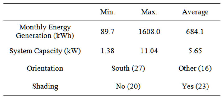
Table 1. Descriptive statistics of forty-three installed solar panels.
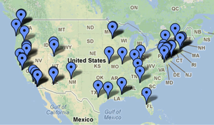
Figure 1. Geographic locations of forty-three individual solar panel systems (Map Data ©2103 Google INEGI Maplink TeleAtlas).
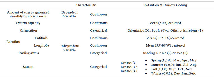
Table 2. Characteristics and definitions of variables.
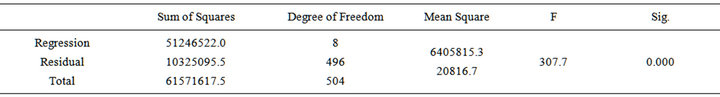
Table 3. ANOVA results.
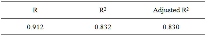
Table 4. Model summary.
systems (R2 = 0.832), and an estimated 83% of the variance in output projected for the population of similar systems (R2 adj. = 0.83).
Based on the results shown in Table 5, a regression equation was found, where the predicted monthly energy generation can be found from the equation: Predicted Energy generation = 912.584 + 124.743 (System Capacity – 5.63) – 29.127 (Orientation D1) – 9.027 (Latitude – 38˚50'N) + 2.743 (Longitude – 95˚40'W) – 50.845 (Shading D1) – 67.054 (Season D1) – 261.658(Season D2) – 394.221 (Season D3). As shown by the t values and the corresponding significance values, all of the slopes are statistically significant (i.e., we can conclude at the 0.05 level that all slopes are not zero). Hence, all the independent variables contribute in predicting the amount of energy generated monthly by the solar panels included in the sample. Since none of the independent variables has a variance inflation factor (VIF) greater than five, there are no apparent multi-collinearity problems [17]; in other words, there is no variable in the model that measures the same relationship/quantity as is measured by another variable. Moreover, the fitted model was found to not violate other basic assumptions required in a valid regression model. Because the coefficients of the independent variables are all significant at the 0.05 level of significance, the average amount of energy generated monthly by the given PV system set may be adjusted as follows by each independent variable, holding other variables constant:
• Monthly energy generation will increase by approximately 125.3 (kWh) for each 1 (kW) increase in the system capacity of the solar panels.
• For the given geographic region, solar panels facing south will generate as much as 29.1 (kWh) more energy than solar panels facing other orientations.
• Regarding locations within the United States, power generation will be larger in solar panels installed in the western or southern United States than in the eastern or northern United States. This energy generation will increase by 9.0 (kWh) for each 1 degree decrease in latitude and will increase by 2.7 (kWh) for each 1 degree increase from center longitude.
• Shading will reduce the amount of energy generation as much as 50.85 (kWh).
• As expected, solar panels will generate more energy in summer than in other seasons; 67.05, 261.7, and 394.2 more energy (kWh) in summer than in spring, fall, and winter, respectively.
• Regarding the interpretation of the numeric constants in the equation, a solar panel will generate approximately 912.6 (kWh) energy when the system capacity is 5.63 (kW), the panels are facing south, are located at the latitude of 38˚50'N and the longitude of 95˚ 40'W, are not shaded, and during the summer season.
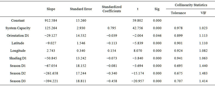
Table 5. Regression coefficients of independent variables.
While the slope coefficients all contribute to the prediction of PV output, the relative importance can be gauged by the Beta, or Standardized Coefficient values given in Table 5. Betas with larger absolute values are more important than those with smaller absolute values given that they are in standard deviation units instead of the varying units of the original independent variables.
5. Discussion and Conclusion
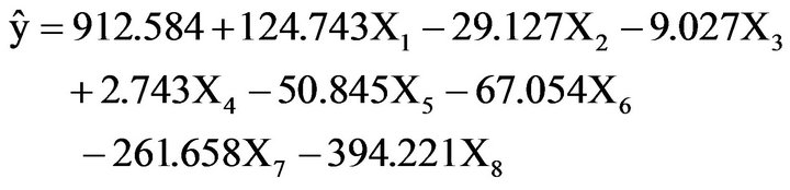
This study examined the relationships between the amount of energy generated monthly by a known set of solar panels and various predictors. Based on a total of 505 energy output data points generated monthly by forty-three solar panels installed in the United States, a regression equation was derived for predicting photo voltaic energy generation of PV systems with a system capacity between 1.4 and 11.0 kW. The monthly energy generation, ŷ, can be predicted from the equation:
where:
• ŷ = Predicted monthly photo voltaic energy generation;
• X1 = System Capacity – 5.63 (in Kw);
• X2 = Orientation (0 for South, 1 for other orientations);
• X3 = Latitude – 38˚50'N;
• X4 = Longitude – 95˚40'W;
• X5 = Shading (No (0) or Yes (1));
• X6 = Season D1 (Spring, 0 or 1);
• X7 = Season D2 (Fall, 0 or 1);
• X8 = Season D3 (Winter, 0 or 1).
By entering a value for each of the variables X1-X8, users can obtain energy predictions for prospective installations within the range of the systems sampled in this study. In such applications, the regression model developed herein explains over 83% of the variation typically seen in solar PV systems in the US. Moreover, given that the overall model is statistically significant, it is reasonable to assume that the given regression equation can accurately predict the PV output with the parameters described above.
The equation is presented as a practical, simple prediction of small-scale PV system energy generation and an explanation of critical considerations required for solar PV installations. This model will prove helpful to individuals with little experience in solar power systems who may be considering less than optimum conditions for a PV panel installation.
Proper system capacity may be determined depending on a required amount of energy generated monthly and yearly, as well as a given system location, orientation, and shading status. To generate equivalent energy amounts, PV systems in the eastern or northern United States should have larger system capacities than western or southern areas. Additionally, solar panels not facing directly south, or shaded, should have a larger system capacity in order to produce an equivalent output. Additionally, the Beta values produced in the regression analysis provide guidance regarding the importance of the criteria that can be used to further refine the decision making process. Of primary concern is the system capacity. Next, seasonal variation substantially impacts PV output, followed by longitude and then latitude. It is interesting to note that shading and orientation do not appear as variables of central importance. In fact, orientation has a significance value just slightly lower than the 0.05 probability threshold. These relatively low values for orientation and shading may be attributable to relatively small amounts of variation as well as general installation considerations for PV systems. For these variables, while in general there may be small departures from ideal installations, both the installer and the owner have vested interests in approximating ideal conditions. It is difficult to imagine either party tolerating large amounts of shading, or large departures from southerly orientation, so as to maximize solar exposure. Therefore, given the expense and effort required for the installation of systems like those sampled in this study, one would expect that care has been taken to obtain good solar exposure.
The regression model developed in this study can be beneficially utilized by perspective owners of PV solar systems to evaluate the claims of manufacturers and installers relative to a model prediction based from a sample of previously installed systems. Such a comparison can assist perspective owners to better assess both returns on their investment (ROI) and payback periods associated with proposed systems.
6. Limitations and Future Work
This study did not address the variation in PV output associated with system manufacturers, actual inverter efficiencies, and system downtime. Systems produced by different manufacturers vary with respect to quality and efficiency. Likewise, the quality of inverter efficiencies varies widely. Further, the datasets used did not consider discontinuous timelines which would account for system downtime, often attributed to panel damage or failure, inverter failure, weather damage, switch failures, or operator error. Additionally, isolated regions of non-typical cloud cover and solar insolation were not accounted for. Similarly, certain longitudes in the US contained no data sets with continuous energy generation output.
The model generally considered only smaller (1.4 to 11 Kw), grid connected PV systems in capacity sizes common to residential, privately owned PV systems. In comparison with isolated systems, grid-connected systems would be expected to have higher efficiencies due to load balancing. All the energy generated by the PV systems in this study is assumed to be used in grid connected systems where there is always a load greater than the power produced. Isolated, residential systems operating off the grid may utilize all available generated capacity, but must be load balanced.
REFERENCES
- J. L. Lee and S. Y. Kim, “Enhanced Efficiency of Organic Photovoltaic Cells with Sr2SiO4:Eu2+ and SrGa2S4: Eu2+ Phosphors,” Organic Electronics, Vol. 14, No. 4, 2013, pp. 1021-1026. doi:10.1016/j.orgel.2013.01.032
- X. Zhang, X. Zhao, S. Smith, J. Xu and X. Yu, “Review of R&D Progress and Practical Application of the Solar Photovoltaic/Thermal (PV/T) Technologies,” Renewable and Sustainable Energy Reviews, Vol. 16, No. 1, 2012, pp. 599-617. doi:10.1016/j.rser.2011.08.026
- P. Biwole, P. Eclache and F. Kuznik, “Phase-Change Materials to Improve Solar Panel’s Performance,” Energy and Buildings, Vol. 62, 2013, pp. 59-67. doi:10.1016/j.enbuild.2013.02.059
- A. M. Paudel and H. Sarper, “Economic Analysis of a Grid-Connected Commercial Photovoltaic System at Colorado State University-Pueblo,” Energy, Vol. 52, 2013, pp. 289-296.
- P. Denholm and R. Margolis, “The Regional Per-Capita Solar Electric Footprint for the United States,” National Renewable Energy Laboratory, Golden, 2007. doi:10.2172/921203
- S. Danov, J. Carbonell, J. Cipriano and J. Martí-Herrero, “Approaches to Evaluate Building Energy Performance from Daily Consumption Data Considering Dynamic and Solar Gain Effects,” Energy and Buildings, Vol. 57, 2013, pp. 110-118. doi:10.1016/j.enbuild.2012.10.050
- J. K. Kaldellis and A. Kokala, “Quantifying the Decrease of the Photovoltaic Panels’ Energy Yield Due to Phenomena of Natural Air Pollution Disposal,” Energy, Vol. 35, No. 12, 2010, pp. 4862-4869. doi:10.1016/j.energy.2010.09.002
- K. A. Moharram, M. S. Abd-Elhady, H. A. Kandil and H. El-Sherif, “Influence of Cleaning Using Water and Surfactants on the Performance of Photovoltaic Panels,” Energy Conversion and Management, Vol. 68, 2013, pp. 266-272. doi:10.1016/j.enconman.2013.01.022
- G. Boyle, “Renewable Energy: Power for A Sustainable Future,” Oxford University Press, Oxford, 2004.
- F. Cucchiella and I. D’Adamo, “Estimation of the EnerGetic and Environmental Impacts of a Roof-Mounted Building-Integrated Photovoltaic Systems,” Renewable and Sustainable Energy Reviews, Vol. 16, No. 7, 2012, pp. 5245-5259. doi:10.1016/j.rser.2012.04.034
- NREL, “PVWatts Software,” National Renewable Energy Laboratory, Golden, 2013. http://rredc.nrel.gov/solar/calculators/pvwatts/version1
- D. Thevenard and S. Pelland, “Estimating the Uncertainty in Long-Term Photovoltaic Yield Predictions,” Solar Energy, Vol. 91, 2013, pp. 432-445. doi:10.1016/j.solener.2011.05.006
- T. Oozeki, T. Izawa, K. Otani and K. Kurokawa, “An Evaluation Method of PV Systems,” Solar Energy Materials and Solar Cells, Vol. 75, No. 3-4, 2003, pp. 687-695. doi:10.1016/S0927-0248(02)00143-5
- S. Mau and U. Jahn, “Performance Analysis of GridConnected PV Systems,” 21st European Photovoltaic Solar Energy Conference, Dresden, 4-8 September 2006.
- B. Marion, J. Adelstein, K. Boyle, H. Hayden, B. Hammond, T. Fletcher, B. Canada, D. Narang, D. Shugar, H. Wenger, A. Kimber, L. Mitchell, G. Rich and T. Townsend, “Performance Parameters for Grid-Connected PV Systems,” 31st IEEE Photovoltaics Specialists Conference and Exhibition, Lake Buena Vista, 3-7 January 2005, pp. 1601-1606.
- T. Hong, C. Koo and M. Lee, “Estimating the Loss Ratio of Solar Photovoltaic Electricity Generation through Stochastic Analysis,” ICCEPM, Garden Grove, 9-11 January 2013, pp. 389-399.
- R. O’Brien, “A Caution Regarding Rules of Thumb for Variance Inflation Factors,” Quality & Quantity, Vol. 41, No. 5, 2007, pp. 673-690. doi:10.1007/s11135-006-9018-6