Open Journal of Statistics
Vol. 3 No. 5 (2013) , Article ID: 37644 , 7 pages DOI:10.4236/ojs.2013.35036
A Class of Truncated Binomial Lifetime Distributions
Department of Quantitative Analysis, King Saud University, Riyadh, KSA
Email: salkarni@ksu.edu.sa
Copyright © 2013 Said Hofan Alkarni. This is an open access article distributed under the Creative Commons Attribution License, which permits unrestricted use, distribution, and reproduction in any medium, provided the original work is properly cited.
Received July 16, 2013; revised August 16, 2013; accepted August 23, 2013
Keywords: Lifetime Distributions; Decreasing Failure Rate; Binomial Distribution
ABSTRACT
In this paper, a new lifetime class with decreasing failure rate is introduced by compounding truncated binomial distribution with any proper continuous lifetime distribution. The properties of the proposed class are discussed, including a formal proof of its probability density function, distribution function and explicit algebraic formulae for its reliability and failure rate functions. A simple EM-type algorithm for iteratively computing maximum likelihood estimates is presented. The Fisher information matrix is derived in order to obtain the asymptotic covariance matrix. This new class of distributions generalizes several distributions which have been introduced and studied in the literature.
1. Introduction
The study of life length of organisms, structures, materials, etc., is very important in the biological and engineering sciences. A substantial part of such study is devoted to modeling the lifetime data by a failure distribution. The exponential, Rayleigh, and Weibull distributions are the most commonly used distributions in reliability and life testing. These distributions have several desirable properties and nice physical interpretations. Unfortunately, however, the exponential and Rayleigh distributions have constant and increasing failure rates, respectively. The Weibull distribution generalizes both these distributions which may have increasing, constant, or decreasing failure rates.
Multi-parameter distributions to model lifetime data have been introduced by compounding a continuous lifetime and power series distributions. The exponential geometric (EG), exponential Poisson (EP) and exponential logarithmic distributions were introduced and studied by (Adamidis and Loukas [1]), (Kus [2]) and (Tahmasbi and Rezaei [3]), respectively. Recently, (Chahkandi and Ganjali [4]) introduced the exponential power series (EPS) distributions, which contain these distributions.
Situations where the failure rate function decreases with time have been reported by several authors. Indicative examples are business mortality (Lomax [5]), failure in the air-conditioning equipment of a fleet of Boeing 720 aircrafts or in semiconductors from various lots combined (Proschan [6]) and the life of integrated circuit modules (Saunders and Myhre [7]). In general, a population is expected to exhibit decreasing failure rate (DFR) when its behavior over time is characterized by “work hardening” (in engineering terms) or “immunity” (in biological terms); sometimes the broader term “infant mortality” is used to denote the DFR phenomenon. The resulting improvement of reliability with time might have occurred by means of actual physical changes that caused self-improvement or simply it might have been due to population heterogeneity. Indeed, (Proschan [6]) provided that the DFR property is inherent to mixtures of distributions with constant failure rate (see also (McNolty et al. [8]) for other properties of exponential mixtures and (Gleser [9]) demonstrated the converse for any gamma distribution with shape parameter less than one. In addition, (Gurland and Sethuramm [10]) give examples illustrating that such results may hold for mixtures of distributions with rapidly increasing failure rate. A mixture of truncated geometric distribution and exponential with DFR was introduced by (Adamidis and Loukas [11]). The exponential-Poisson (EP) distribution was proposed by (Kus [2]), and generalized by (Hemmati et al. [12]) using Wiebull distribution and the exponential-logarithmic distribution was discussed by (Tahmasbi and Rezaei [3]). (Silvia et al. [13]) did a new distribution with decreasing, increasing and upside down bathtub failure rate. A twoparameter distribution family with decreasing failure rate arising by mixing power-series distribution has been introduced by (Chahkandi and Ganjali [4]). A Weibull power series class of distributions with Poisson was presented by (Morais and Barreto-Souza [14]). (Morais [15]) in a master degree thesis presented a class of generalized Beta distributions, Pareto power series and Weibull power series. Lately, (Alkarni and Oraby [16]) and (Alkarni [17]) obtained a class of truncated Poisson and logarithmic distributions with any continuous lifetime distribution.
A further exponentiated type distribution has been introduced and studied in the literature. The exponentialWeibull (EW) distribution was proposed by (Mudholkar and Srivastava [18]) to extend the GE distribution. This distribution was also studied by (Mudholkar et al. [19]), (Mudholkar and Hutson [20]) and (Nassar and Eissa [21]). (Nadarajah and Kotz [22]) introduced four more exponentiated type distributions: the exponentiated gamma, exponentiated Weibull, exponentiated Gumbel and exponentiated Fréchet distributions by generalizing the gamma, Weibull, Gumbel and Fréchet distributions in the same way that the GE distribution extends the exponential distribution. (Barreto-Souza and Cribari-Neto [23]) introduced the generalized exponential-Poisson distribution which extends the exponential-Poisson distribution in the same way that the GE distribution extends the exponential distribution.
In this paper we generalize the work of (Bakouchetal. [24]) to a class of several lifetime continuous distributions and hence any mixture of continuous lifetime with truncated binomial distribution such as exponential, Weibull, pareto becomes a special case of this class. This paper is organized as follow. In Section 2, the new class of binomial lifetime distributions with its probability and distribution functions is introduced. In Section 3, the corresponding survival and hazard rate functions with some of their properties are derived. In Section 4, maximum likelihood estimate of the unknown parameters is obtained based on a random sample via EM algorithm. In Section 5, the entropy for the binomial lifetime distributions class is discussed.
2. The Class
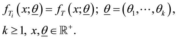
Given  let
let  be independent and identically distributed (iid) random variables with probability density function (pdf) given by
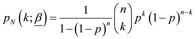
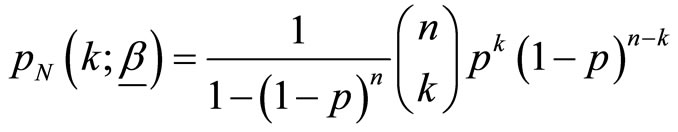
Here,  is a zero truncated binomial random variable with probability mass function given by

where  with
with ,
,  and
and 
 are independent. Let
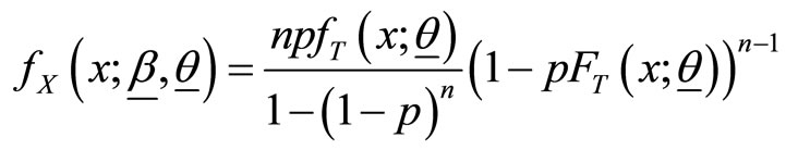
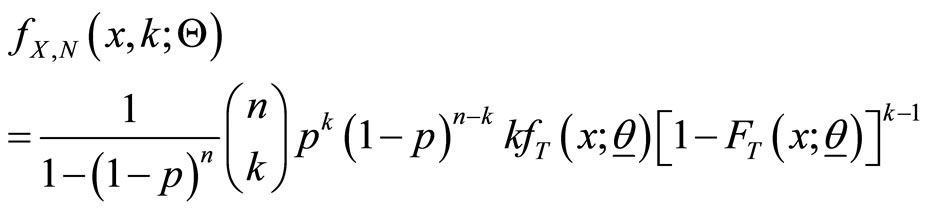
 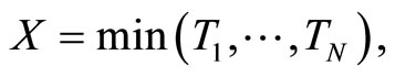 then, the pdf of the random variable
  is obtained as
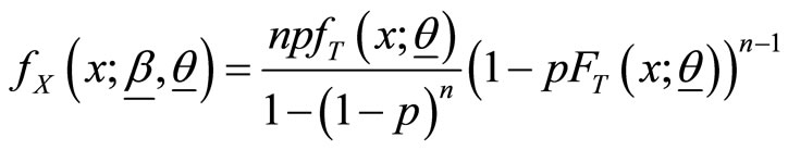 (1)
(1)
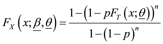
And hence the cumulative distribution function (cdf) of  is
is
 (2)
(2)
The proof of the results in (1) and (2) are presented in the following theorem.
Theorem 2.1 Suppose  with
with

and  is a zero truncated binomial random variable with probability mass function
and  with
with  where
where  and
and  are independent. If
  then the pdf and cdf of
  are
are
and
respectively.
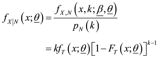
Proof: By definition, the pdf of  given
given  is
is
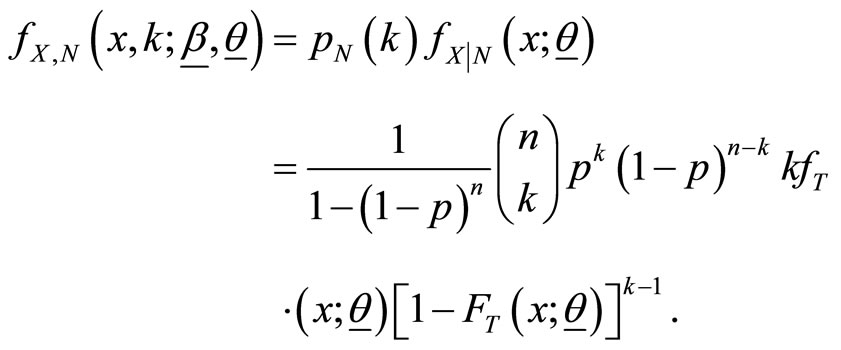
and hence the joint pdf of  and
and  is obtained as
The marginal pdf and cdf of are given by
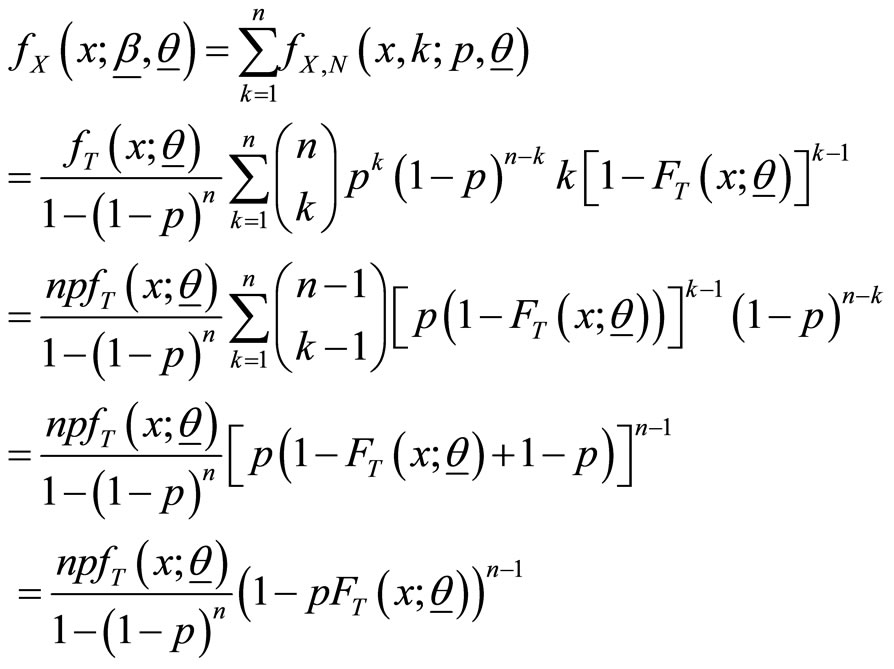
and
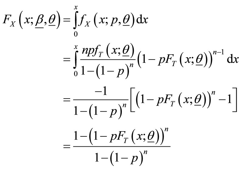
respectively.
We denote a random variable  with pdf and cdf (1) and (2) by
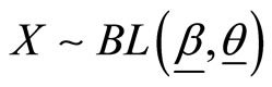 . This new class of distributions generalizes several distributions which have been introduced and studied in the literature. For instance using the probability density and its distribution function of exponential distribution in (1), we obtain the binomial exponential distribution (Bakouch et al. [24]) and using Wiebull probability density and its distribution function gives binomial Wiebull distribution (Morais and BarretoSouza ([14]). The model is obtained under the concept of population heterogeneity (through the process of compounding). An interpretation of the proposed model is as follows: a situation where failure (of a device for example) occurs due to the presence of an unknown number,
  of initial defects of same kind (a number of semiconductors from a defective lot, for example). The Ts represent their lifetimes and each defect can be detected only after causing failure, in which case it is repaired perfectly (Adamidis and Loukas [1]). Then, the distributional assumptions given earlier lead to any of the BL distributions for modeling the time to the first failure
 .
.
Table 1 shows the probability function and the distribution function for some lifetime distributions.
Some lifetime distributions are excluded from this table such as Gamma and lognormal distribution stable since they do not have closed forms. They still can be applied in this class numerically.
The  quantile
  of the BL distribution, the inverse of the distribution function
 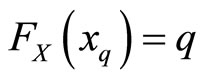 is the same as the inverse of the distribution function
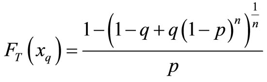
for any continuous lifetime with distribution function 
3. Survival and Hazard Functions
Since the BL is not part of the exponential family, there is no simple form for moments see for instant (Kus [2]) for the exponential case. Survival function (also known reliability function) (sf) and hazard function (known as failure rate function) (hf) for the BL class are given in the following theorem.
Theorem 3.1 Suppose that  with
with


Table 1. Probability and distribution functions.
and  is a zero truncated binomial random variable with probability mass function
and  with
with  where
where  and
and  are independent. If
  then the sf and hf of
  are
are
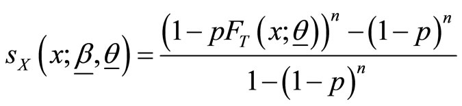 , (3)
, (3)
and
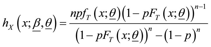 , (4)
, (4)
Respectively.
Proof: Using (1) and (2), survival function (also known reliability function) and hazard function (known as failure rate function) for the BL class are given respectively by
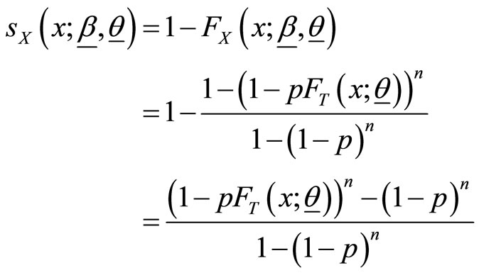
and
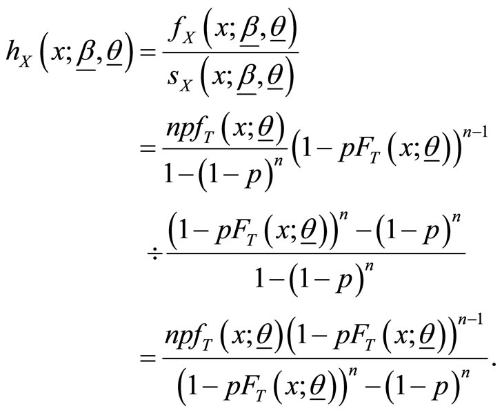
Table 2 summarizes the survival functions and hazard rate functions for some distributions of the class.
The hazard function for BL class is decreasing because the DFR property follows from the result of (Barlow et al. [25]) on mixtures.
4. Estimation
In what follows, we discuss the estimation of the BL class parameters. Let,  be a random sample with observed values
  from a BL distributions with parameters
  and
and . Let
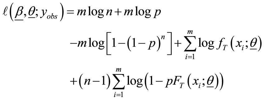
. Let  be the parameters vector. The log-likelihood function based on the observed random sample size of
  is obtained by
and the associated score function is given by
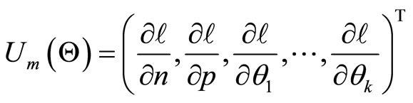 where
where
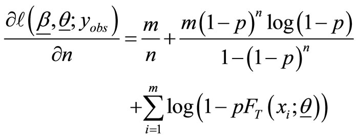 (5)
(5)
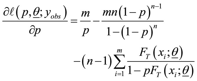 (6)
(6)
and
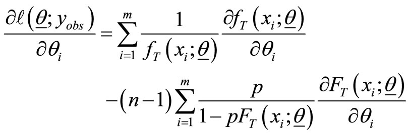 (7)
(7)
For 
The maximum likelihood estimates(MLE) of , say
, say , is obtained by solving the nonlinear system
  The solution of this nonlinear system of equations has not a closed form, but can be found numerically by using software such as MATHEMATICA, MAPLE, Ox and R.
For interval estimation and hypothesis tests on the model parameters, we require the information matrix. The  information matrix is
  where the elements of
  are the second partial derivatives of (5), (6) and (7). Under the regular conditions stated in (Cox and Hinkley [26]), that are fulfilled for our model whenever the parameters are in the interior of the parameter space, we have that the asymptotic distribution of
  is multivariate normal
 , where
  is the unit information matrix.

Table 2. Survival and hazard functions.
EM Algorithm
Based on the underline distribution, the maximum likelihood estimation of the parameters can be found analytically using an EM algorithm. Newton-Raphson algorithm is one of the standard methods to determine the MLEs of the parameters. To employ the algorithm, second derivatives of the log-likelihood are required for all iteration. EM algorithm is a very powerful tool in handling the incomplete data problem (Dempster et al., [27]; McLachlan and Krishnan, [28]). It is an iterative method by repeatedly replacing the missing data with estimated values and updating the parameter estimates. It is especially useful if the complete data set is easy to analyze. As pointed out by (Little and Rubin [29]), the EM algorithm will converge reliably but rather slowly (as compared to the Newton-Raphson method) when the amount of information in the missing data is relatively large. Recently, EM algorithm has been used by several authors such as (Adamidis and Loukas [1]), (Adamidis [30]), (Ng et al. [31]), (Karlis [32]) and (Adamidis et al. [11]).
To estimate , EM algorithm is a recurrent method such that each step consists of an estimate of the expected value of a hypothetical random variable and later maximizes the log-likelihood of the complete data. Let the complete data be
  with observed values
  and the hypothetical random variable
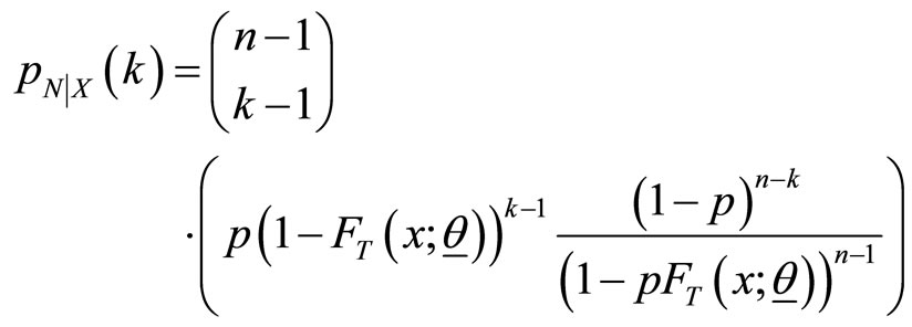
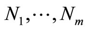 . The joint probability function is such that the marginal density of
  is the likelihood of interest. Then, we define a hypothetical complete-data distribution for each
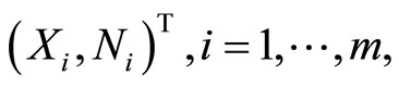
With a joint probability function in the form
With  and
and . Thus, it is straight forward to verify that the E-step of an EM cycle requires the computation of the conditional expectation of
 , where
  is the current estimate (in the rth iteration) of
 . The EM cycle is completed with M-step, which is complete data maximum likelihood over
 , with the missing N’s replaced by their conditional expectations
  (Adamidis and Loukas [1]), where
and its expected value is
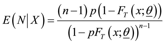 .
.
5. Entropy for the Class
If  is a random variable having an absolutely continuous cumulative distribution function
  and probability distribution function
  then the basic uncertainty measure for distribution
  (called the entropy of
 ) is defined as
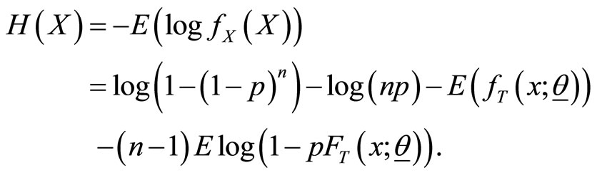 (8)
(8)
Statistical entropy is a probabilistic measure of uncertainty or ignorance about the outcome of a random experiment, and is a measure of a reduction in that uncertainty. Since Shannon’s [33] pioneering work on the mathematical theory of communication, entropy (8) has been used as a major tool in information theory and in almost every branch of science and engineering. Numerous entropy and information indices, among which there is the Renyi entropy, have been developed and used in various disciplines and contexts. Information theoretic principles and methods have become integral parts of probability and statistics and have been applied in various branches of statistics and related fields.
6. Acknowledgements
The author is highly grateful to the deanship of scientific research at King Saud University represented by the research center at college of business administration for supporting this research financially.
REFERENCES
- K. Adamidis and S. Loukas, “A Lifetime Distribution with Decreasing Failure Rate,” Statistics and Probability Letters, Vol. 39, No. 1, 1998, pp. 35-42.
- C. Kus, “A New Lifetime Distribution,” Computational Statistics and Data Analysis, Vol. 51, 2007, pp. 4497- 4509.
- R. Tahmasbi and S. Rezaei, “A Two-Parameter Lifetime Distribution with Decreasing Failure Rate,” Computational Statistics and Data Analysis, Vol. 52, 2008, pp. 3889- 3901.
- M. Chahkandi and M. Ganjali, “On Some Lifetime Distributions with Decreasing Failure Rate,” Computational Statistics and Data Analysis, Vol. 53, 2009, pp. 4433- 4440.
- K. Lomax, “Business Failures: Another Example of the Analysis of Failure Data,” Journals of American Statistical Association, Vol. 49, 1954, pp. 847-852.
- F. Proschan, “Theoretical Explanation of Observed Decreasing Failure Rate,” Journal of Technometrics, Vol. 5, 1963, pp. 375-383.
- S. Saunders and J. Myhre, “Maximum Likelihood Estimation for Two-Parameter Decreasing Hazard Rate Distributions Using Censored Data,” Journals of American Statistical Association, Vol. 78, 1983, pp. 664-673.
- F. McNolty, J. Doyle and E. Hansen, “Properties of the Mixed Exponential Failure Process,” Technometrics, Vol. 22, 1980, pp. 555-565.
- L. Gleser, “The Gamma Distribution as a Mixture of Exponential Distributions,” Journals of American Statistical Association, Vol. 43, 1989, pp. 115-117.
- J. Gurland and J. Sethuraman, “Reversal of Increasing Failure Rates When Pooling Failure Data,” Technometrics, Vol. 36, 1994, pp. 416-418.
- K. Adamidis, T. Dimitrakopoulou and S. Loukas, “On an Extension of the Exponential-Geometric Distribution,” Statistics & Probability Letters, Vol. 73, 2005, pp. 259- 269.
- F. Hemmati, E. Khorram and S. Rezakhah, “A New ThreeParameter Distribution,” Journal of Statistical Planning and Inference, Vol. 141, 2011, pp. 2255-2275.
- R. Silva, W. Barreto-Souza and G. Cordeiro, “A New Distribution with Decreasing, Increasing and Upside-Down Bathtub Failure Rate,” Computational Statistics & Data Analysis, Vol. 54, 2010, pp. 935-944.
- A. Morais and W. Barreto-Souza, “A Compound Class of Weibulland Power Series Distributions,” Computational Statistics and Data Analysis, Vol. 55, 2011, pp. 1410- 1425.
- A. Morais, “A Class of Generalized Beta Distributions, Pareto Power Series and Weibull Power Series,” M.s. Thesis, Universidade Federal de Pernambuco, Recife-PE, 2009.
- S. Alkarni and A. Oraby, “A Compound Class of Poisson and Lifetime Distributions,” Journal of Statistics Applications & Probability, Vol. 1, 2012, pp. 45-51.
- S. Alkarni, “New Family of Logarithmic Lifetime Distributions,” Journal of Mathematics and Statistics, Vol. 8, No. 4, 2012, pp. 435-440.
- G. Mudholkar and D. Srivastava, “Exponentiated Weibull Family for Analyzing Bathtub Failure-Rate Data,” IEEE Transaction on Reliability, Vol. 42, 1993, pp. 299-302.
- G. Mudholkar, D. Srivastava and M. Freimer, “The Exponentiated Weibull Family,” Journal of Technometrics, Vol. 37, 1995, pp. 436-445.
- G. Mudholkar and A. Hutson, “The Exponentiated Weibull Family: Some Properties and a Flood Data Application,” Communications in Statistics, Theory and Methods, Vol. 25, 1996, pp. 3059-3083.
- M. Nassar and F. Eissa, “On the Exponentiated Weibull Distribution,” Communications in Statistics, Theory and Methods, Vol. 32, 2003, pp. 1317-1336.
- S. Nadarajah and S. Kotz, “The Beta Exponential Distribution,” Reliability Engineering and System Safety, Vol. 91, 2006, pp. 689-697.
- W. Barreto-Souza and F. Cribari-Neto, “A Generalization of the Exponential-Poisson Distribution,” Statistics & Probability Letters, Vol. 79, 2009, pp. 2493-2500.
- H. Bakouch, M. Ristic, A. Asgharzadah and L. Esmaily, “An Exponentiated Exponential Binomial Distribution with Application,” Statistics and Probability Letters, Vol. 82, 2012, pp. 1067-1081.
- R. Barlow, A. Marshall and F. Proschan, “Properties of Probability Distributions with Monotone Hazard Rate,” The Annals of Mathematical Statistics, Vol. 34, 1963, pp. 375-389.
- D. Cox and D. Hinkley, “Theoretical Statistics,” Chapman and Hall, London, 1974.
- A. Dempster, N. Laird and D. Rubin, “Maximum Likelihood from Incomplete Data via the EM Algorithm,” Journal of The Royal Statistical Society Series B, Vol. 39, 1977, pp. 1-38.
- G. McLachlan and T. Krishnan, “The EM Algorithm and Extension,” Wiley, New York, 1997.
- R. Little and D. Rubin, “Incomplete Data,” In: S. Kotz and N. L. Johnson, Eds., Encyclopedia of Statistical Sciences, Vol. 4, Wiley, New York, 1983.
- K. Adamidis, “An EM Algorithm for Estimating Negative Binomial Parameters,” Austral, New Zealand Statistics, Vol. 41, No. 2, 1999, pp. 213-221.
- H. Ng, P. Chan and N. Balakrishnan, “Estimation of Parameters from Progressively Censored Data Using EM Algorithm,” Computational Statistics & Data Analysis, Vol. 39, 2002, pp. 371-386.
- D. Karlis, “An EM Algorithm for Multivariate Poisson Distribution and Related Models,” Journal of Applied Statistics, Vol. 301, 2003, pp. 63-77.
- C. Shannon, “A Mathematical Theory of Communication,” Bell System Technical Journal, Vol. 27, 1948, pp. 379- 432.