ABSTRACT

This paper considers quantile regression analysis based on semi-competing risks data in which a non-terminal event may be dependently censored by a terminal event. The major interest is the covariate effects on the quantile of the non-terminal event time. Dependent censoring is handled by assuming that the joint distribution of the two event times follows a parametric copula model with unspecified marginal distributions. The technique of inverse probability weighting (IPW) is adopted to adjust for the selection bias. Large-sample properties of the proposed estimator are derived and a model diagnostic procedure is developed to check the adequacy of the model assumption. Simulation results show that the proposed estimator performs well. For illustrative purposes, our method is applied to analyze the bone marrow transplant data in [1].

1. Introduction

Quantile regression analysis has received increasing attentions in the recent literature of survival analysis. Compared with conventional regression models such as the proportional hazards (PH) model or the accelerated failure time (AFT) model, quantile regression models provide direct assessment of the covariate effect on different quantiles of the failure time variable. This model also allows covariates to affect both location and shape of the distribution. Let T be the failure time of interest, be a vector and. Consider the following linear quantile regression model on, where is a known monotonic function, such that

(1)

where and is the th quantile of Y conditional on Z. Note that when we set, model (1) is equivalent to . Many papers for estimating without specifying the distribution of or have appeared in the literature. [2-5] considered quantile regression analysis under a fixed censoring mechanism in which all the censoring times are observed. Independent right censorship has been assumed by many papers including [6-11].

In this paper, we consider semi-competing risks data [12] in which the failure time of a non-terminal event T is subject to dependent censoring by a terminal event time D but not vice versa. Consider an example of bone marrow transplantation for leukemia patients described in [1] such that T is the time to leukemia relapse and D is the time to death. One important risk factor is the disease classification (i.e. ALL, AML low-risk, and AML highrisk) which was determined based on patient’s status at the time of transplantation. Here we assume that T, the time to a non-terminal event, follows model (1). Note that [13,14] also considered quantile regression analysis for competing risks data and left-truncated semi-competing risks data respectively. They defined the quantiles based on the crude quantity, namely the cumulative incidence function. In contrast, the proposed regression model (1) is defined based on the net quantity which is not identifiable without extra assumption on the dependence structure. There has been some controversy over which quantity should be used in presence of dependent competing risks. We believe that both quantities are important and not mutually exclusive as they provide information on different aspects of the data. Here measures the covariate effect on T after separating the potential influence from D. Such analysis is also useful in practical applications. For example, a covariate may prolong D so that increase but have no direct effect on the nonterminal event. The dependence between T and D complicates the estimation of. We will adopt a semi-parametric copula assumption to model their joint distribution and apply the technique of inverse probability weighting (IPW) to correct the bias due to dependent censoring in the estimation procedure. The association parameter in the copula model will also be estimated using existing methods.

The rest of this paper is organized as follows. In Section 2, we introduce the data structure and model assumptions. The proposed methodology for parameter estimation and model checking is presented in Section 3. The proofs of the asymptotic properties are given in the Appendix. Section 4 contains simulation results. In Section 5, we apply the proposed methods to analyze the bone marrow transplant data in [1] and in Section 6, we give some concluding remarks.

2. Data and Model Assumptions

Recall that T and D denote the time to a non-terminal event and the time to a terminal event respectively such that T is subject to censoring by D but not vice versa. In presence of additional external censoring due to drop-out or the end-of-study effect, one observes such that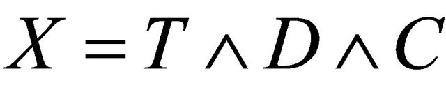, , , , 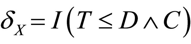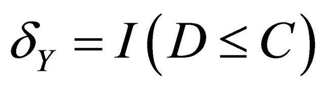where is the minimum operator and is the indicator function. The covariate vectors can be denoted as and. The sample Contains which are random replications of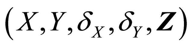. We will assume that and C are independent given Z. The covariate effect on T is specified by model (1) and the major objective is to estimate based on semi-competing risks data.

To handle dependent censoring, we have to make extra assumptions about the dependence structure between T and D in the upper wedge. According to [15] who extended Sklar’s theorem to the regression setting, we consider the following copula model

(2)

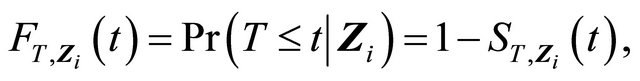
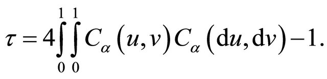
where, and are the marginal survival functions of T and D, given, and is a parametric copula function defined on the unit square. The association parameter in (2) is related to Kendall’s tau defined by

In particular, we will assume in the upper wedge follows a popular subclass of copula models, namely Archimedean copula (AC), in which the copula function can be further expressed as

(3)

where is a non-increasing convex function defined on with. Examples of Archimedean copula include Clayton’s copula with

and

;

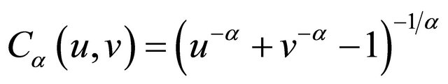and Frank’s copula with

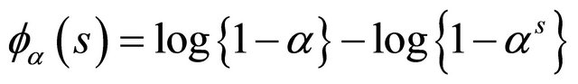
and

.

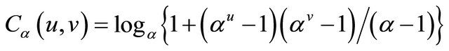3. The Proposed Inference Methods

Our major objective is to develop an inference method for estimation but, in the mean time, employ existing methods for estimating based on semicompeting risks data such as those proposed by [16] and [17].

3.1. Estimation of for Discrete Covariates

In absence of censoring, one can estimate by solving

Since is subject to censoring by, it follows that

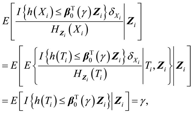
where the reciprocal of the weight function is given by

The above derivations yield the following estimating function for

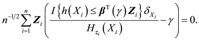
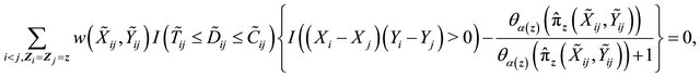
This is the so called inverse probability weighting technique for bias correction. Since needs to be estimated, it is natural to modify the estimating equation as

(4)

where the estimated components in the weight can be denoted as

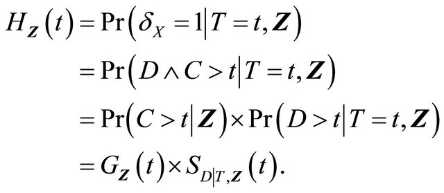
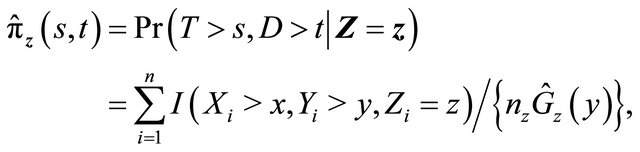
Now we discuss estimation of the weight components. We will first address the situation that Z takes discrete values, and then briefly discuss possible modification for continuous covariates. Since is independent of T and D given Z, can be estimated by the Kaplan-Meier estimator based on data

or

with. We will utilize some analytic properties of the chosen AC model to derive an explicit expression of. Denote,

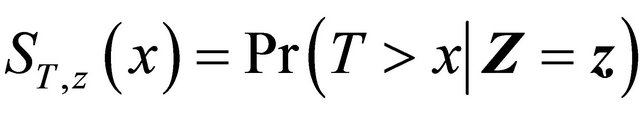and

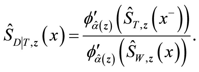
. It follows that

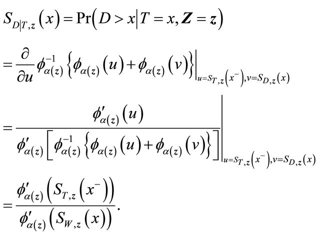
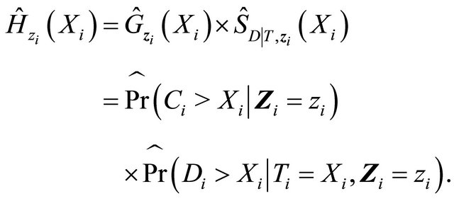
We suggest to estimate by applying the estimators in [17] for quantities in the right-hand side of the above expression. Specifically is the Kaplan-Meier estimator of based on

, where,

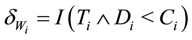is the copula-graphic estimator

where the estimator is the root of the following estimating equation,

where, , ,

, , is a weight function, 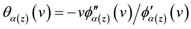, and

where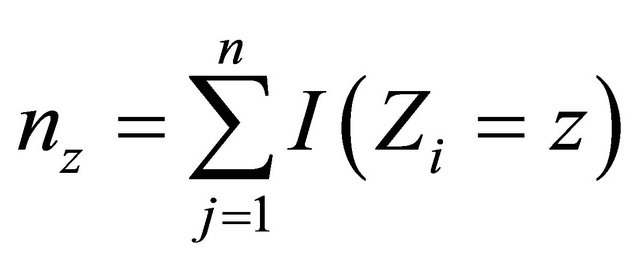. Then

(5)

This estimator is then used in estimating Equation (4).

The Equation (4) may not be continuous so that an exact solution may not exist. Here we define as a generalized solution as in [13,18]. By the monotonic property of (4), the set of generalized solutions is convex. Using the arguments in [13], the solution of (4) can be reformulated as the minimizer of the following function,

where M is a large enough positive value to bound

and from above.

We suggest using a re-sampling approach for variance estimation since the analytic formula for the variance of is complicated to calculate. Based on the nonparametric bootstrap approach, we can sample replications from the original data. Given a bootstrap sample, we can compute. Repeating the re-sampling procedure B times, we obtain

and the variance of can be estimated by

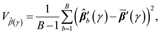
where. Furthermore, we can construct the confidence interval for as

, where, and

is the cumulative distribution function of a standard normal random variable. The bootstrap percentile method suggests another way of constructing a confidence interval of with the formula

, where,

are the order statistics of for.

3.2. Asymptotic Properties for Discrete Covariates

We establish the uniform consistency and weak convergence of the proposed estimator for, a region that is identifiable. We first state the regularity conditions.

(C1) Denote the set of possible covariate Z values as which is a compact set in. The probability density function for covariate Z is uniformly bounded above and below on.

(C2) There exists a compact set in the parameter space for the copula parameter such that all true values of are interior points of for all.

(C3) There exists such that, , and

.

(C4) 1) is Lipschitz continuous for;

2) The density is bounded above uniformly for and; 3) The copula generator function has continuous derivatives,

, , and which do not equal 0 for all and.

(C5) eigmin, for some

and, where,

and for a vector u.

Condition C1 assumes the boundedness of covariates and is satisfied for finite discrete covariates. This assumption is only used to derive the asymptotic properties of for proving Theorem 1. Condition C2 assumes that the true value of is an interior point in the parameter space which is a common regularity condition. Condition C3 is assumed to simplify theoretical arguments similar to condition C1 in [13], and generally is the study end time in practical applications. Conditions C4 1) and 2) assume the smoothness of coefficient processes, and the uniform boundedness on the density of T, which are standard for quantile regression methods. Condition C4 3) imposes the smoothness requirement on the copula generator function similar to the regularity conditions in [17,19]. Condition C5 is similar to condition C4 in [13] which ensures the identifiability of and is needed for proving the consistency of.

Therefore with finite, we prove the following result.

Theorem 1 If conditions C1-C5 hold, then

and converges weakly to a meanzero Gaussian process.

The detailed proofs are presented in the Appendix.

3.3. Model Checking and Model Diagnosis

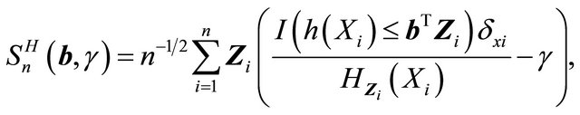
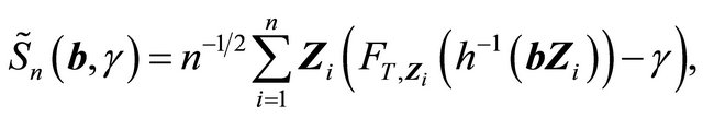
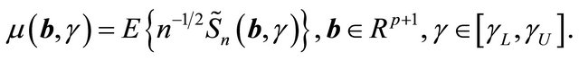
Motivated by the work of [20-22] in which complete data are considered, we define the residual quantities as

for and consider

where is a known bounded weight function. Similar to the arguments in [13,23], converges weakly to a zero-mean Gaussian process if model (1) is specified correctly and the covariate takes discrete values. Therefore we propose the following test statistic

where is an estimator of the standard deviation of which can be obtained by applying the bootstrap approach mentioned earlier. Thus, we have that T_n converges to the standard normal random variable asymptotically as the model is correct. On the other hand, when the model is mis-specified, T_n will deviate from zero. Accordingly we can reject the model assumption if, where is the quantile of and is the level of significance. If there are K candidate models under consideration, we compute the absolute value of T_n for each model for and choose the one with the smallest value.

3.4. Estimation for Continuous Covariates

We briefly discuss how to extend our estimation method for continuous covariates. One can apply a smoothing approach to estimate the probability functions conditional on z. Following [24], without loss of generality, assume that and are ordered. Let

where, is the bandwidth and is the kernel. Then

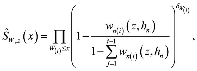
where are the rearrangement sorted according to W_i, where and

, and is the copula-graphic estimator in [24]

(6)

and solves estimating equation

Special techniques are needed to derive the asymptotic properties for the case of continuous covariates. For example properties of the smoothed versions of and are not fully available yet. The convergence rate for the normality proof may not be directly extended since the smooth version of may not be asymptotic normal. However the estimator for the quantile regression parameter may still be asymptotic normal even when some component converges at a slower rate.

4. Simulation Studies

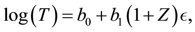
We conduct simulation studies to examine the finitesample performance of the proposed methods with R software. Here we consider two cases. For the first one, we consider the model,

(7)

where and. We generate which follow the Clayton copula and Frank copula with marginally following so that, and D marginally following exp(2). For the second case, we consider

(8)

where, and generated from the Clayton copula and Frank copula with following and. In this case,. Three levels of association τ = 0.3, 0.5, 0.7 are considered. The censoring variable C follows a uniform distribution on.

We evaluate the performances for γ = 0.1, 0.3, 0.5 and the sample size n = 100 based on 400 simulation runs. To obtain the standard error of the proposed estimator, we use the bootstrap method with B = 50. Based on the settings, we also present a naive estimator of, which is constructed under the wrong assumption that T is independently censored by. That is, we estimate by solving the estimating Equation (4) with

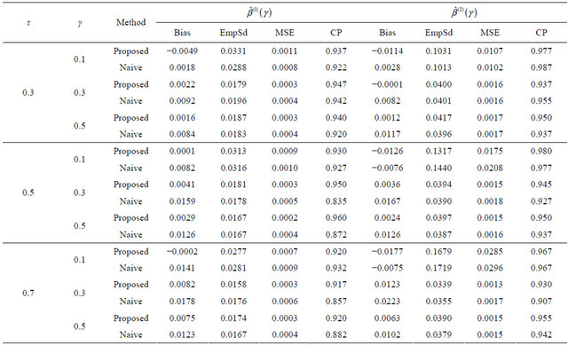
Tables 1-4 report the average bias of the proposed

Table 1. Finite-sample results for estimating the quantile regression parameters under model (7) with Clayton copula.

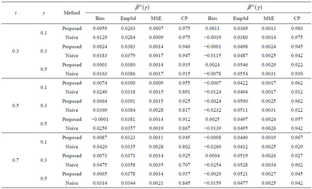
The results are based on 400 simulation runs each with a sample size 100.

Table 2. Finite-sample results for estimating the quantile regression parameters under model (8) with Clayton copula.

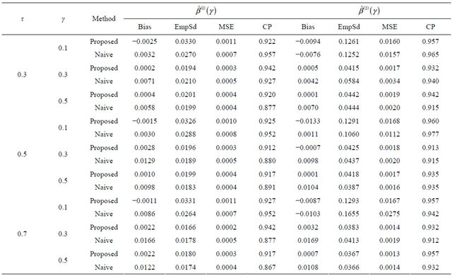
The results are based on 400 simulation runs each with a sample size 100.

Table 3. Finite-sample results for estimating the quantile regression parameters under model (7) with Frank copula.

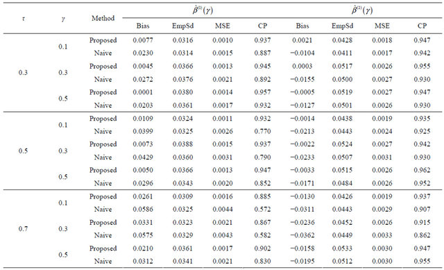
The results are based on 400 simulation runs each with a sample size 100.

Table 4. Finite-sample results for estimating the quantile regression parameters under model (8) with Frank copula.

The results are based on 400 simulation runs each with a sample size 100.

point estimator, , (Bias);

the empirical standard deviation,

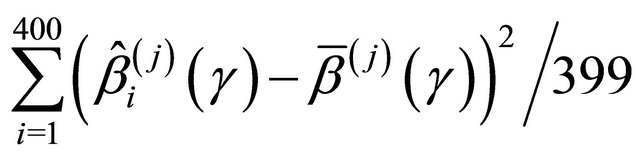where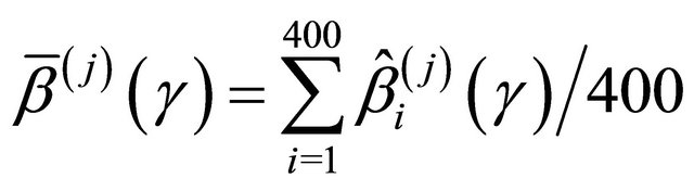, (EmpSd); the mean squared error, Bias² + EmpSd², (MSE); and the coverage probability of the 95% confidence intervals,

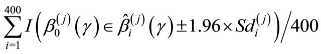where is the estimated standard deviation of by the bootstrap approach, (CP). From the results, we can see that our proposed estimator has much smaller bias and smaller mean squared error than the naive estimator. The confidence intervals coverage probabilities are close to the nominal level 95% in most cases while the naive estimator has the coverage rate far below the nominal level in many cases. Although the proposed estimator of has the coverage rate lower than 90% in the first case with Kendall’s tau τ = 0.7 but it still performs better than the naive estimator. As the sample size increases to n = 200 for that case (data omitted here), the coverage probabilities for proposed estimator become close to the nominal level while the coverage probabilities for the naive estimator get worse. This confirms that our estimator is asymptotically correct while the naive estimator is not.

Then we examine the proposed model diagnostic method when the true model is generated from

where, , and

so that and

follow Clayton copula with. We consider  τ = 0.3, 0.5, 0.7 and γ = 0.1, 0.3, 0.5 under n = 100 based on 200 replications.

Three forms of transformation are fitted: 1) ; 2); 3). Table 5

presents the rejection probabilitywhere α = 0.05, and the probability that the fitted model is selected as the one which gives the smallest value of among the three candidates. From the results, we see that when, the rejection probability (type-I error rate) is close to the specified level of α = 0.05. When the fitted model is wrong, the rejection probability (power of the test) is very high in most cases.

Table 5. Finite-sample results for the proposed model checking method.

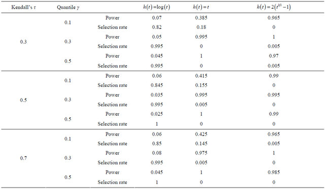
Note: The sample size is 100 and replications are 200. “Power” =, where. “Selection rate” is the proportion that the fitted model is selected as the one giving the smallest value of among the three candidates.

Even for the case where the power is relatively low around 40% (the γ = 0.1 quantile for), the probabilities of selecting the correct model are still high.

5. Data Analysis

We apply the proposed methodology to analyze the bone marrow transplant data based on 137 leukemia patients provided by [1]. Patients were classified into three risk categories: ALL, AML low-risk, and AML high-risk based on their status at the time of transplantation. The covariates (Z₁, Z₂) are coded as ALL (Z₁ = 1, Z₂ = 0), AML low-risk (Z₁ = 1, Z₂ = 0), and AML high-risk (Z₁ = 0, Z₂ = 1). We want to investigate how the risk classification is related to the quantile of the relapse time. Specifically the fitted model is given by

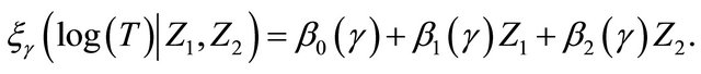(9)

The results are summarized in the Tables 6 and 7 based on B = 1000 bootstrap replications. Table 6 contains the estimators and model checking tests with 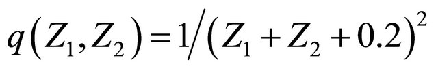. The p-value is the testing result by the model checking approach provided in SubSection 3.3. Since all the p-values are greater than 0.05, we adopt the model in (9) for further analysis.

From the analysis we see that patients of AML lowrisk had longer relapse time than those in the other two groups and the difference is more obvious for those with earlier relapse. For example, the 10% quantile of the relapse time in the AML low-risk group is 3.2964 times of that in ALL group and 4.751 times of that in AML highrisk group. The group differences are statistically significant for the 10% and 30% quantiles. but no longer significant for the 50% quantile.

6. Concluding Remarks

In this paper, we consider quantile regression analysis for analyzing the failure-time of a non-terminal event under the semi-competing risks setting. The Archimedean copula assumption is adopted to specify the dependency between the two correlated events. This assumption is utilized to calculate the weight for bias correction in the estimation of quantile regression parameters. Here we focus on the case of discrete covariates and derive the asymptotic properties of the proposed estimators. The bootstrap method is suggested for variance estimation. For checking the adequacy of the fitted model, a model diagnostic approach is proposed. Simulation results confirm that the proposed methods have good performances in finite samples. In the data analysis, we see that the risk classification is particularly influential for earlier relapse. The methodology can be extended to allow for continuous covariates by employing some smoothing techniques but the corresponding theoretical analysis is beyond the scope of the paper.

Table 6. Estimation of quantile regression parameters and model checking test based on the bone marrow transplant data.

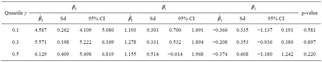
Table 7. Comparison of leukemia relapse time for the three risk groups.

7. Acknowledgement

This paper was financially supported by the National Science Council of Taiwan (NSC100-2118-M-194-003- MY2).

REFERENCES

Appendix: Proofs of Theorem 1

The proof follow the outline similar to the proof in [13]. The technical details need to be adjusted for dependent censoring which make things harder.

Define

For simplicity, we use and to denote supremum taken over, and respectively.

First, we show that converges uniformly to

. Since is finite, as

. Hence by [17], is consistent for for all. Using this and conditions C2, it implies that with probability 1 for large enough n. From condition C3, and converge to

and uniformly for. Condition C4 (iii) together with conditions C1 and C3 ensure the uniform boundedness of the first two derivatives of and for and

, same as the regularity condition in [19]. Hence as, by [17] and [19], also converges to uniformly for. Then there exists a number such that and fall into with probability 1 for large enough n and all by condition C3 and the uniform convergence of the two estimators. Denote. Condition C4 (iii)

implies that, and

are all uniformly bounded above for and. Hence

converges to

uniformly for and. This result and the uniform convergence of imply the uniform convergence of for and. Hence we have

The function class

is Donsker because the class of indicator functions is Donsker and both and are uniformly bounded by conditions C1 and C3. Therefore, by Glivenko-Cantelli theorem, . Also

(1)

Then the consistency of comes from the identifiability condition C5 using the arguments in the proof of Theorem 1 in [13].

Similar to [13] the following lemma holds with the uniform boundedness of Z, and that comes from conditions C1, C3 (i) and C3 (ii).

Lemma 1. For any positive sequence satisfying,

Now, we provide the proof for the asymptotic normality of. One can write

From the uniform convergence and asymptotic weak convergence of and condition C3, we have for any r > 0. Hence the above quantity is dominated by the first term. By Lemma 1 and the uniform convergence of to,

where denotes asymptotic equivalence uniformly in. Applying Taylor expansions for at, and using the uniform convergence of to, we have

where. Since,

(2)

It remains to prove the weak convergence of to a zero-mean Gaussian process. It follows that

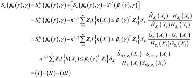
The first two terms (I) and (II) can be proved to converge to zero-mean Gaussian processes by applying the arguments in [13] as follows. The family

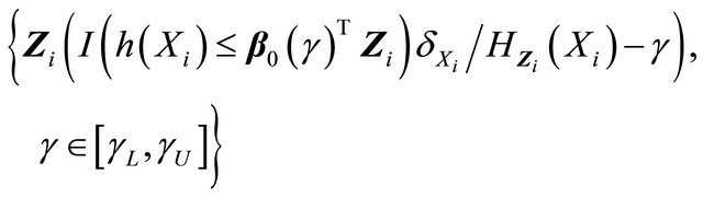
is Donsker by the Lipschitz continuity of (condition C4 (i)) and uniformly boundedness of and (conditions C1 and C3). Thus, the first term

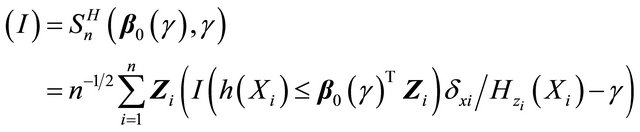
converges weakly to a zero-mean Gaussian process.

Denote and as the at-risk processes at time t. Let

,

,

..

Then 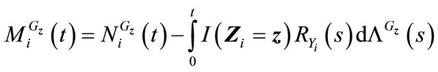is a martingale.

From martingale representation theory for univariate independent censoring,

So the second term can be written as

where.

From uniform boundedness of, and, it is easy to show that

is Lipschitz in b. Then similarly can be shown to be Donsker, and the second term also converges weakly to a zero-mean Gaussian process.

For the third term, recall

with. Denote

,

and

.

So for,

For notation brevity, denote

,

and

.

The third term becomes

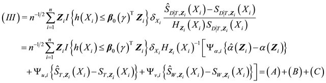
Since is finite, by condition C1 for all. So with follows a Gaussian distribution. Let

Now term is

which follows a Gaussian distribution by the boundedness of and.

Denote

,

.

Denote

where

.

.

Then

is a martingale. Then

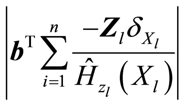
Now similar to the martingale expression for the second term, we have term as

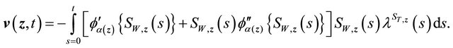
where

.

Similar as (II) above, is Lipschitz in b, and 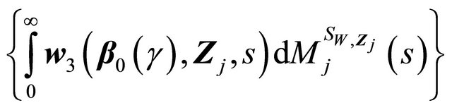is Donsker. Thus the term (B) converges weakly to a zero-mean Gaussian process.

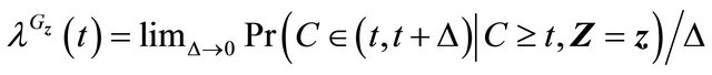
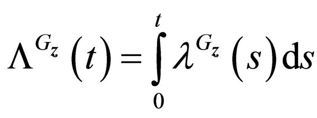
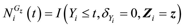
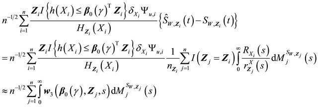
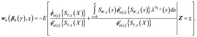
Finally, for term, let

be the crude hazard function in [17],

.

.

Then

is a martingale. From [17], we have

where

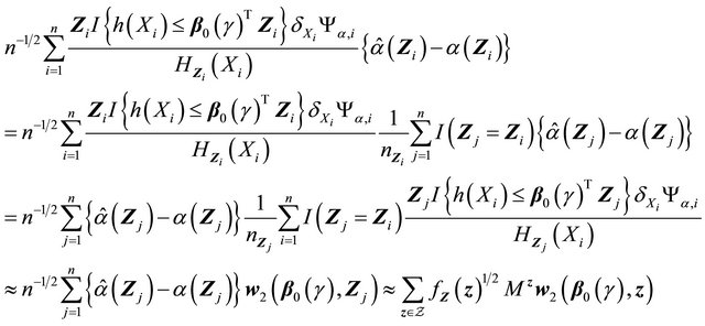
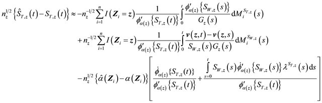
Similar to terms (A) and (B), we have term (C) equals

where

Then each of the three terms in (C) can be shown to converge to zero-mean Gaussian process similarly as above.

Summarizing the results above, converges weakly to a zero-mean Gaussian process. Hence (2) implies that converges weakly to a zero-mean Gaussian process for.

REFERENCES

- J. P. Klein and M. L. Moeschberger, “Survival Analysis: Techniques for Censored and Truncated Data,” 2nd Edition, Springer, New York, 2003.
- J. Powell, “Least Absolute Deviations Estimation for the Censored Regression Model,” Journal of Econometrics, Vol. 25, No. 3, 1984, pp. 303-325. doi:10.1016/0304-4076(84)90004-6
- J. Powell, “Censored Regression Qunatiles,” Journal of Econometrics, Vol. 32, No. 1, 1986, pp. 143-155. doi:10.1016/0304-4076(86)90016-3
- B. Fitzenberger, “A Guide to Censored Quantile Regressions,” In: G. S. Maddala and C. R. Rao, Eds., Handbooks of Statistics, North-Holland, Amsterdam, 1997, pp. 405-437. doi:10.1016/S0169-7161(97)15017-9
- M. Buchinsky and J. Hahn, “A Alternative Estimator for Censored Quantile Regression,” Econometrica, Vol. 66, No. 3, 1998, pp. 653-671. doi:10.2307/2998578
- Z. Ying, S. H. Jung and L. J. Wei, “Survival Analysis with Median Regression Models,” Journal of the American Statistical Association, Vol. 90, No. 429, 1995, pp. 178-184. doi:10.1080/01621459.1995.10476500
- S. Yang, “Censored Median Regression Using Weighted Empirical Survival and Hazard Functions,” Journal of the American Statistical Association, Vol. 94, No. 445, 1999, pp. 137-145. doi:10.1080/01621459.1999.10473830
- S. Portnoy, “Censored Regression Quantiles,” Journal of the American Statistical Association, Vol. 98, No. 464, 2003, pp. 1001-1012. doi:10.1198/016214503000000954
- L. Peng and Y. Huang, “Survival Analysis Based on Quantile Regression Models,” Journal of the American Statistical Association, Vol. 103, No. 482, 2008, pp. 637- 649. doi:10.1198/016214508000000355
- G. Yin, D. Zeng and H. Li, “Power Transformed Linear Quantile Regression with Censored Data,” Journal of the American Statistical Association, Vol. 103, No. 483, 2008, pp. 1214-1224. doi:10.1198/016214508000000490
- S. Portnoy and G. Lin, “Asymptotics for Censored Regression Quantiles,” Journal of Nonparametric Statistics, Vol. 22, No. 1, 2010, pp. 115-130. doi:10.1080/10485250903105009
- J. P. Fine, H. Jiang and R. Chappell, “On Semi-Competing Risks Data,” Biometrika, Vol. 88, No. 4, 2001, pp. 907-919.
- L. Peng and J. P. Fine, “Competing Risks Quantile Regression,” Journal of the American Statistical Association, Vol. 104, No. 488, 2009, pp. 1440-1453. doi:10.1198/jasa.2009.tm08228
- R. Li and L. Peng, “Quantile Regression for Left-Truncated Semicompeting Risks Data,” Biometrics, Vol. 67 No. 3, 2011, pp. 701-710. doi:10.1111/j.1541-0420.2010.01521.x
- A. J. Patton, “Modeling Asymmetric Exchange Rate Dependence,” International Economic Review, Vol. 47, No. 2, 2006, pp. 527-556. doi:10.1111/j.1468-2354.2006.00387.x
- W. Wang, “Estimating the Association Parameter for Copula Models under Dependent Censoring,” Journal of the Royal Statistical Society, Series B, Vol. 65, No. 1, 2003, pp. 257-273. doi:10.1111/1467-9868.00385
- L. Lakhal, L.-P. Rivest and B. Abdous, “Estimating Survival and Association in a Semicompeting Risks Model,” Biometrics, Vol. 64, No. 1, 2008, pp. 180-188. doi:10.1111/j.1541-0420.2007.00872.x
- M. Fygenson and Y. Ritov, “Monotone Estimating Equations for Censored Data,” The Annals of Statistics, Vol. 22, No. 2, 1994, pp. 732-746. doi:10.1214/aos/1176325493
- L.-P. Rivest and M. Wells, “A Martingale Approach to the Copula-Graphic Estimator for the Survival Function under Dependent Censoring,” Journal of Multivariate Analysis, Vol. 79, No. 1, 2001, pp. 138-155. doi:10.1006/jmva.2000.1959
- J. X. Zheng, “A Consistent Nonparametric Regression Models under Quantile Restrictions,” Econometric Theory, Vol. 14, No. 1, 1998, pp. 123-138. doi:10.1017/S0266466698141051
- J. L. Horowitz and V. G. Spokoiny, “An Adaptive, RateOptimal Test of Linearity for Median Regression Models,” Journal of the American Statistical Association, Vol. 97, No. 459, 2002, pp. 822-835. doi:10.1198/016214502388618627
- X. He and L. Zhu, “A Lack-of-Fit Test for Quantile Regression,” Journal of the American Statistical Association, Vol. 98, No. 464, 2003, pp. 1013-1022. doi:10.1198/016214503000000963
- D. Y. Lin and L. J. Wei and Z. Ying, “Checking the Cox Model with Cumulative Sums of Martingle-Based Residuals,” Biometrika, Vol. 80, No. 3, 1993, pp. 557-572. doi:10.1093/biomet/80.3.557
- R. Braekers and N. Veraverbeke, “A Copula-Graphic Estimator for the Conditional Survival Function under Dependent Censoring,” The Canadian Journal of Statistics, Vol. 33, No. 3, 2005, pp. 429-447. doi:10.1002/cjs.5540330308