Open Journal of Statistics
Vol.3 No.4(2013), Article ID:35929,14 pages DOI:10.4236/ojs.2013.34027
Inferences under a Class of Finite Mixture Distributions Based on Generalized Order Statistics
1Department of Mathematics, Assiut University, Assiut, Egypt
2Department of Mathematics, Taif University, Taif, KSA
Email: abahmad2002@yahoo.com, aree.m.z@hotmail.com
Copyright © 2013 Abd EL-Baset A. Ahmad, Areej M. AL-Zaydi. This is an open access article distributed under the Creative Commons Attribution License, which permits unrestricted use, distribution, and reproduction in any medium, provided the original work is properly cited.
Received May 1, 2012; revised January 2, 2013; accepted January 19, 2013
Keywords: Generalized order statistics; Bayes estimation; Heterogeneous population; Monte Carlo Integration; Monte Carlo Simulation
ABSTRACT
The main purpose of this paper is to obtain estimates of parameters, reliability and hazard rate functions of a heterogeneous population represented by finite mixture of two general components. The doubly Type II censoring of generalized order statistics scheme is used. Maximum likelihood and Bayes methods of estimation are used for this purpose. The two methods of estimation are compared via a Monte Carlo Simulation study
1. Introduction
Let the random variable (rv) T follow a class including some known lifetime models, its cumulative distribution function (CDF) is given by
 (1)
(1)
and its probability density function (PDF) is given by
 (2)
(2)
where  is the derivative of
  with respect to t and
  is a nonnegative continuous function of t and
  may be a vector of parameters, such that
 as
as  and
and  as
as 
The reliability function (RF) and hazard rate function (HRF) are given, respectively, by
 (3)
(3)
 (4)
(4)
where
Bayesian inferences based on finite mixture distribution have been discussed by several authors. Bayesian estimation of the mixing parameter, mean and reliability function of a mixture of two exponential lifetime distributions based on right censored samples considered by [1,2] estimated the survival and hazard functions of a finite mixture of two Gompertz components by using type I and type II censored samples, using the maximum likelihood (ML) and Bayes methods. Based on type I censored samples from a finite mixture of two truncated type I generalized logistic components, [3] computed the Bayes estimates of parameters, reliability and hazard rate functions. [4] considered estimation for the mixed exponential distribution based on record statistics. [5] considered Bayes inference under a finite mixture of two compound Gompertz components model. [6] studied some properties of the mixture of two inverse Weibull distributions and obtained the estimates of the unknown parameters via the EM Algorithm.
[7] introduced the generalized order statistics (gos’s). Ordinary order statistics, ordinary record values and sequential order statistics are, among others, special cases of gos’s. The gos’s have been considered extensively by many authors, among others, they are [8-20].
Mixtures of distributions arise frequently in life testing, reliability, biological and physical sciences. Some of the most important references that discussed different types of mixtures of distributions are a monograph by [21-23].
The PDF, CDF, RF and HRF of a finite mixture of two components of the class under study are given, respectively,
 (5)
(5)
 (6)
(6)
 (7)
(7)
 (8)
(8)
where, for , the mixing proportions
  are such that
  and
and are given from (1), (2), (3) after using
  and
and  instead of
  and
and .
.
The property of identifiability is an important consideration on estimating the parameters in a mixture of distributions. Also, testing hypothesis, classification of random variables, can be meaning fully discussed only if the class of all finite mixtures is identifiable. Idenifiability of mixtures has been discussed by several authors, including [24-26].
Our aim of this paper is the estimation of the parameters and functions of these parameters of a class of finite mixture distributions based on doubly Type II censoring gos’s using ML and Bayes methods. Illustrative example of Gompertz distribution is given and compared with the results obtained by previous researchers.
2. Maximum Likelihood Estimation
Let

be the (r - s) gos’s drawn from a mixture of two components of the class (2). Based on this doubly censored sample, the likelihood function can be written [27] as
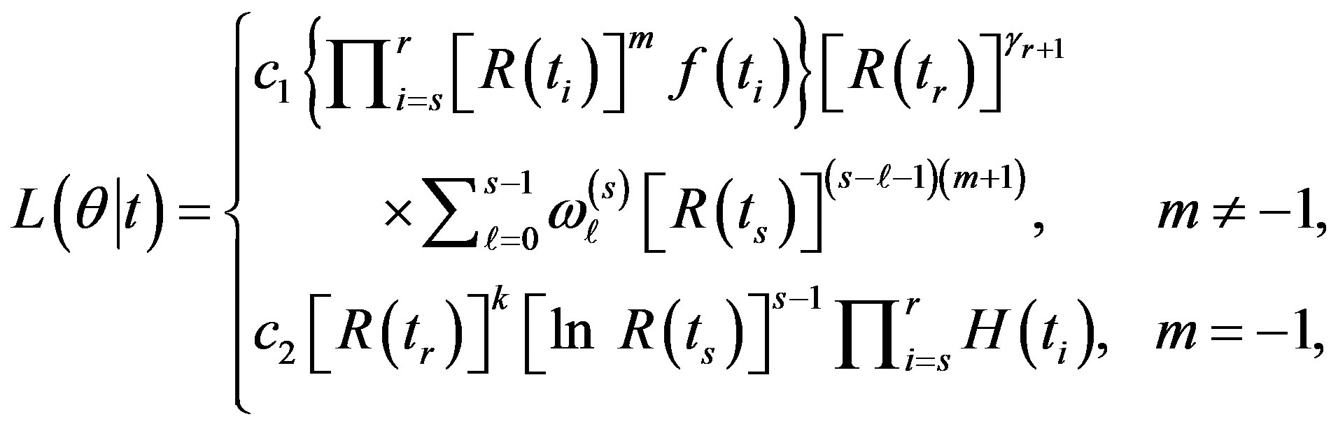 (9)
(9)
where 
 is the parameter space, and
For definition and various distributional properties of gos’s, see [7, 28].
The likelihood function (9) and maximum likelihood estimates (MLE’s) can be obtained by using (1) and (5) in two cases, regarding to m value, as follows.
2.1 MLE’s When 
In this case, substituting (1), (5) in (9), the likelihood function takes the form
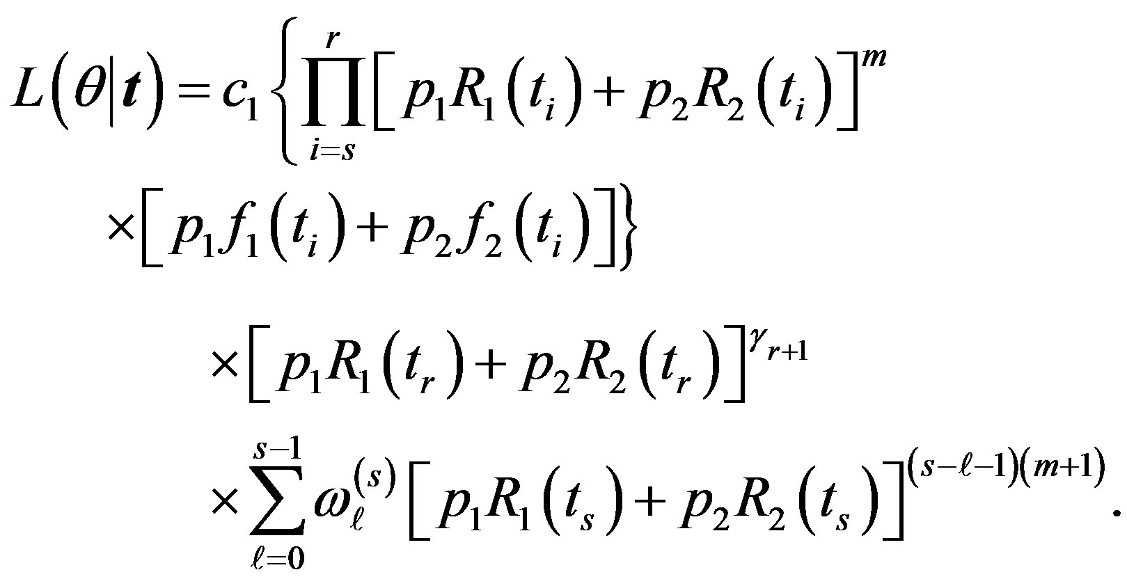 (10)
(10)
Take the logarithm of (10), we have
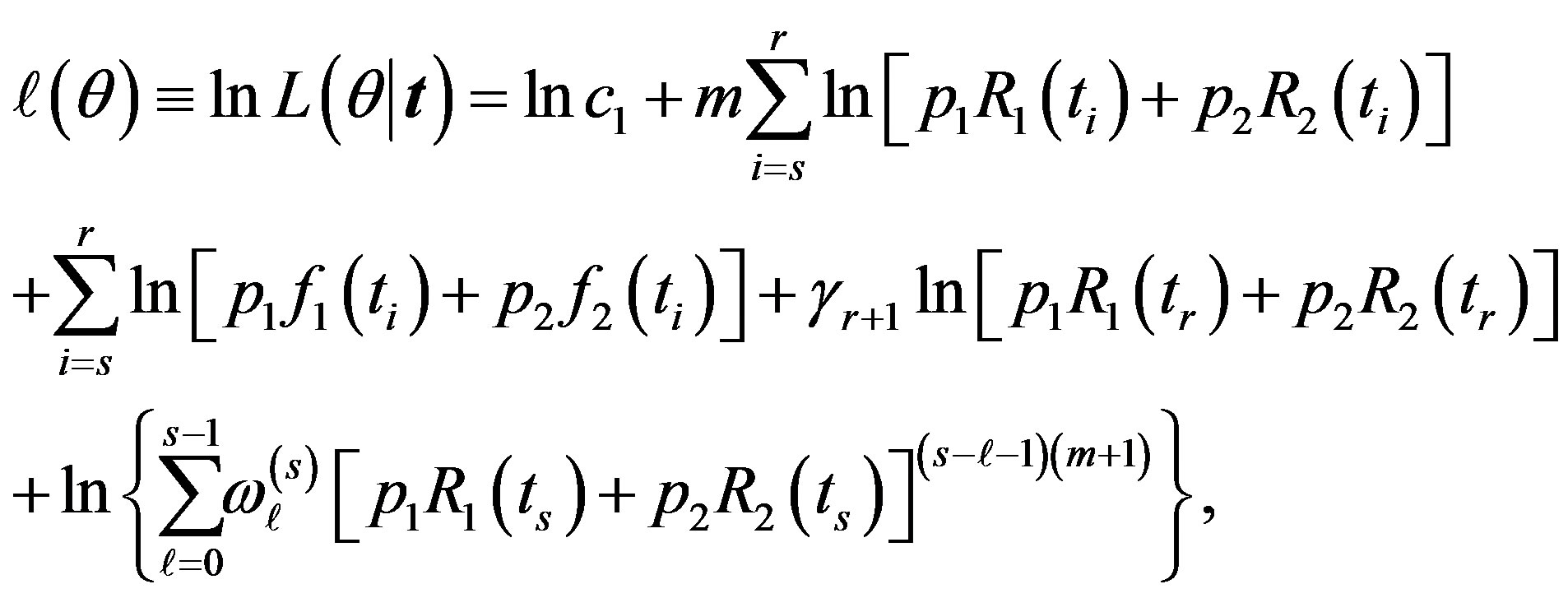 (11)
(11)
where ,
, 
Differentiating (11) with respect to the parameters  and
and  (involved in
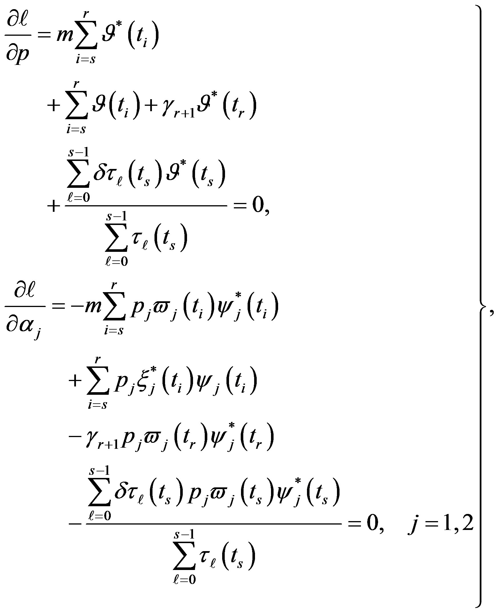
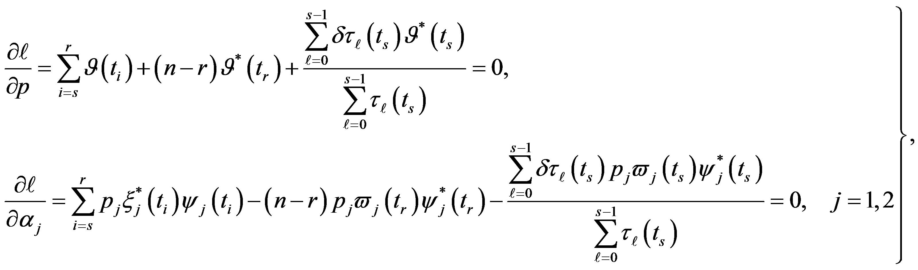
 ) and equating to zero gives the following likelihood equations
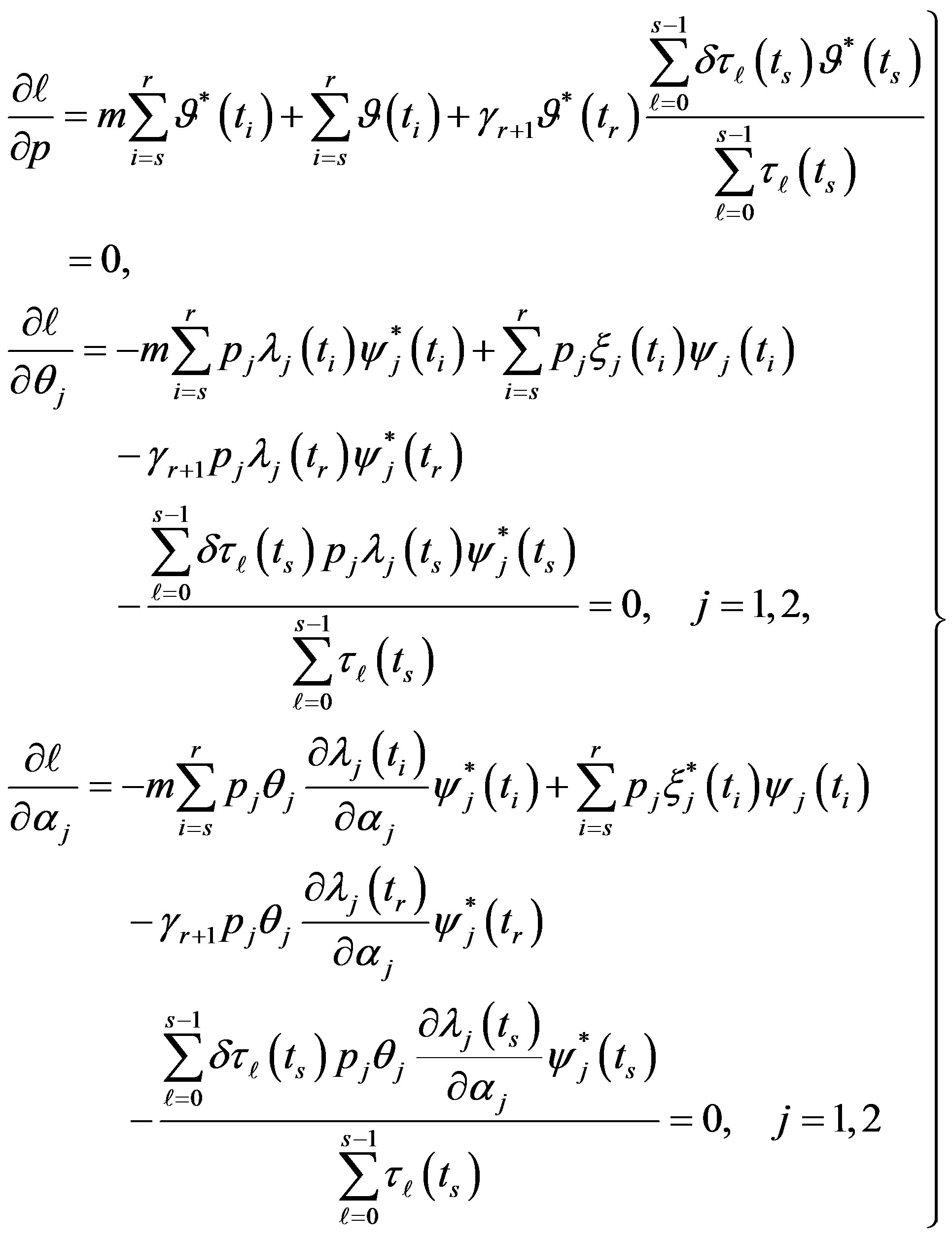 (12)
(12)
where, for j = 1,2
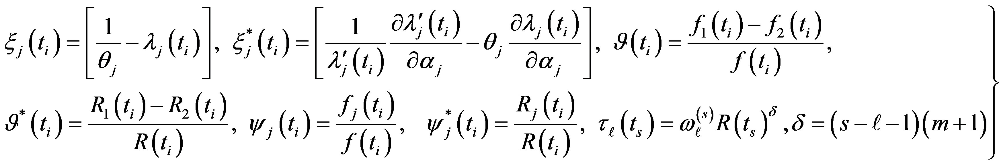 (13)
(13)
The solution of the five nonlinear likelihood Equations (12) using numerical method, yields the MLE’s  and
and .
.
2.2. MLE’s When 
The likelihood function takes the form
 (14)
(14)
So, from (14)
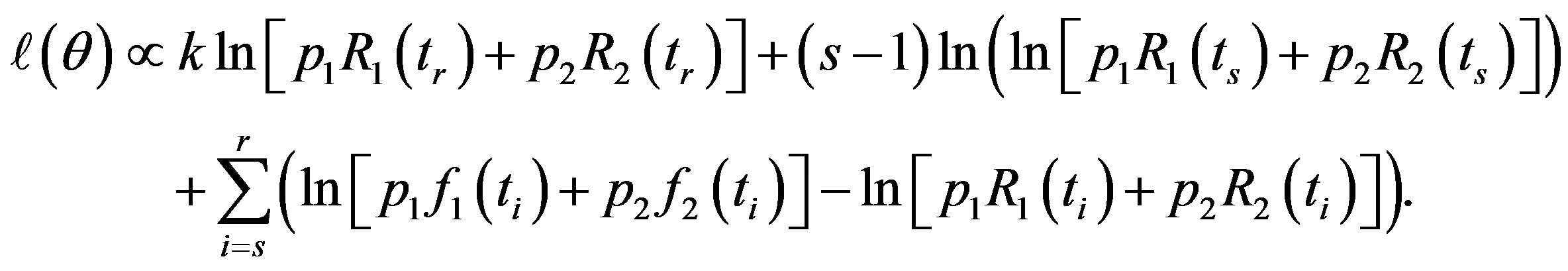 (15)
(15)
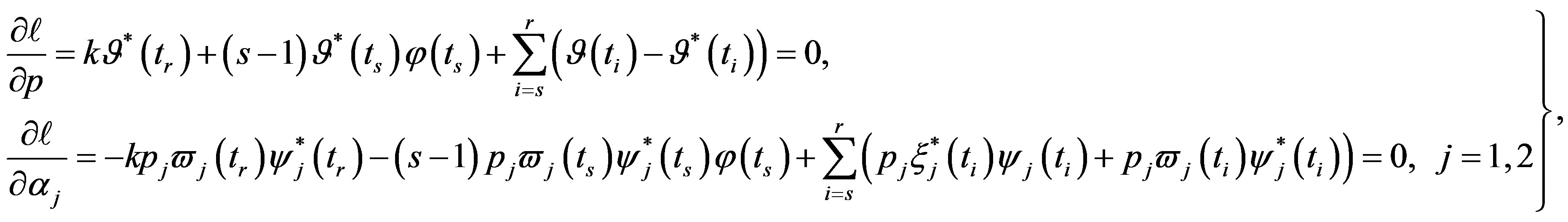
Differentiating (15) with respect to the parameters  and
and  and equating to zero gives the following likelihood equations
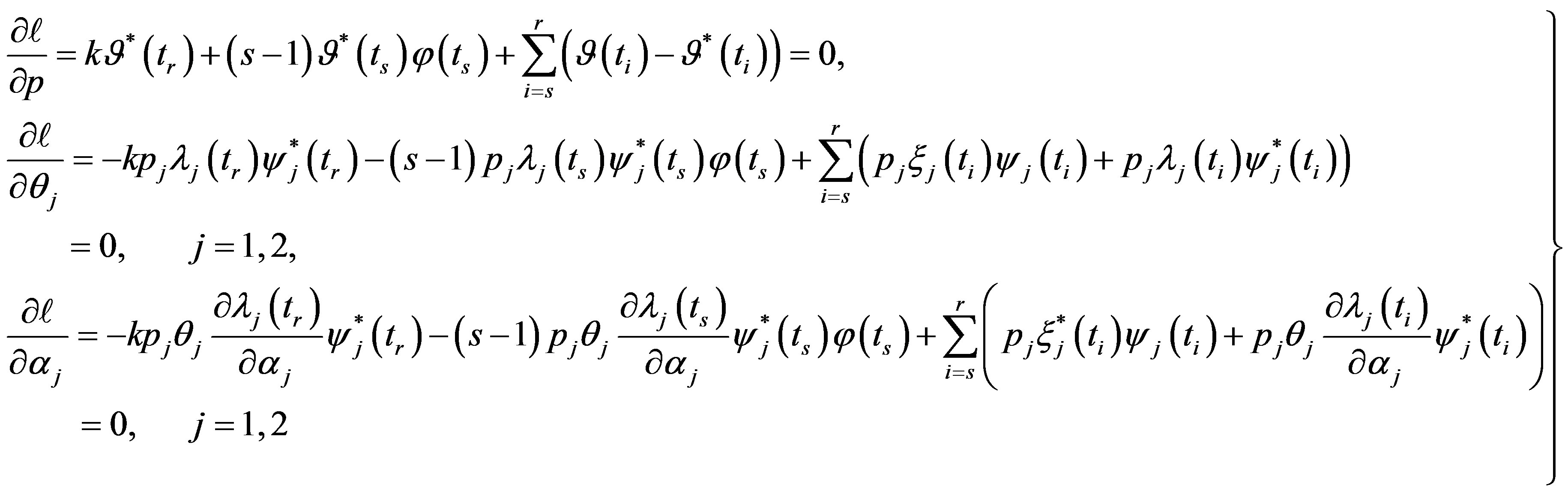 (16)
(16)
where
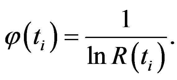 (17)
(17)
The solution of the five nonlinear likelihood Equations (16) using numerical method, yields the MLE’s  and
and .
.
3. Bayes Estimation
In this section, Bayesian estimation for the parameters of a class of finite mixture distributions is considered under squared error and Linex (Linear-Exponential) loss functions.
We shall use the conjugate prior density, that was suggested by [29], in the following form
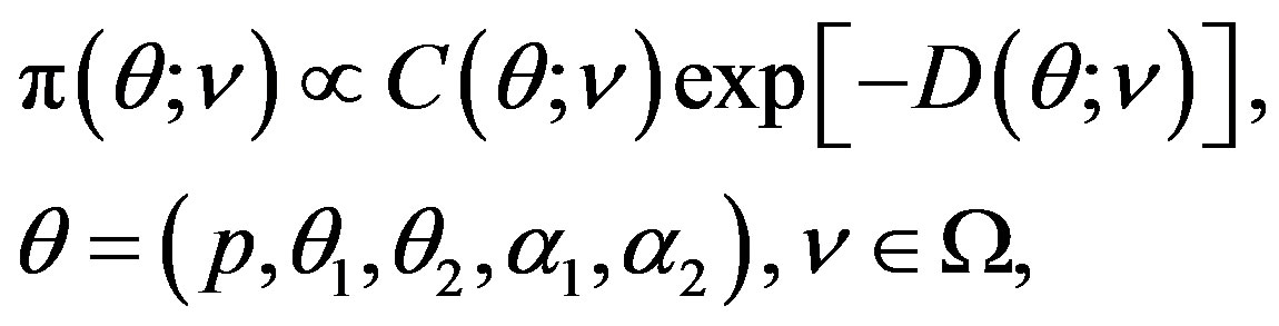 (18)
(18)
where  is the hyperparameter space.
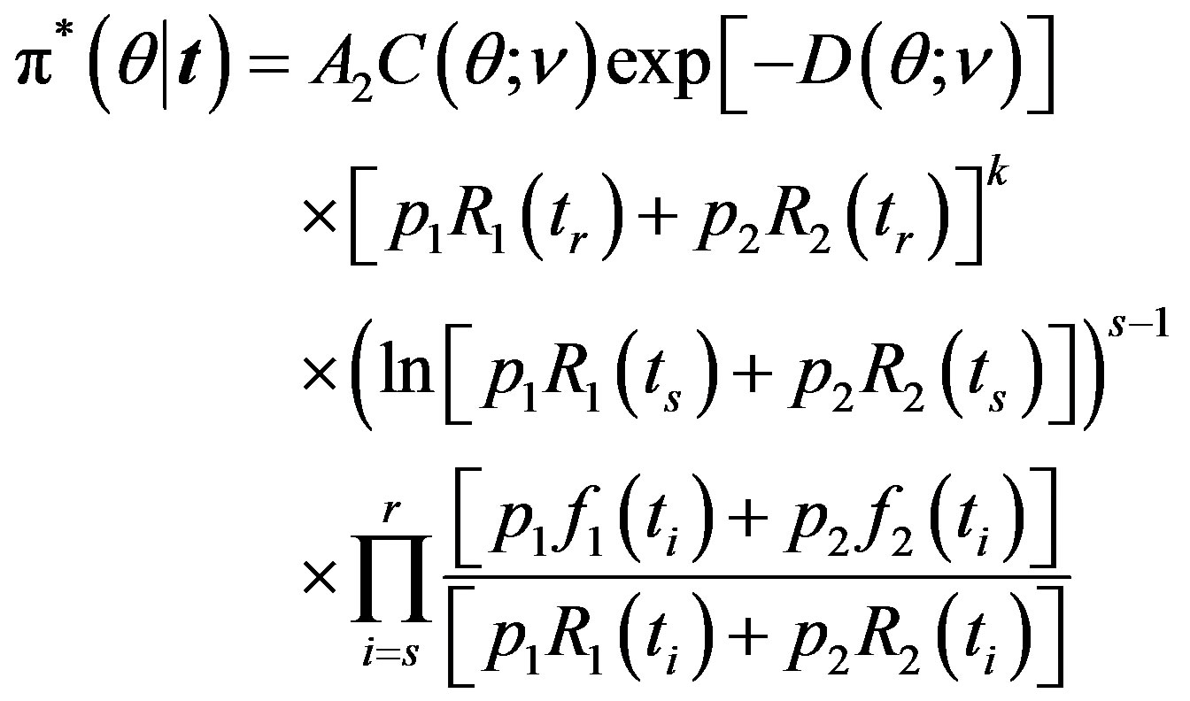
3.1. Bayes Estimates When 
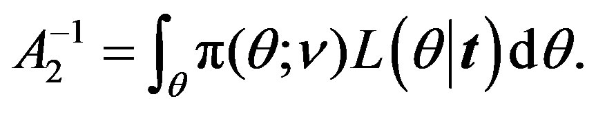
It follows, from (10) and (18), that the posterior density function is given by
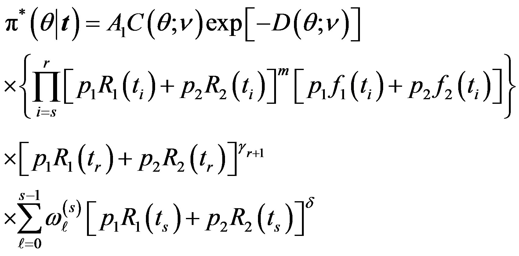 (19)
(19)
where
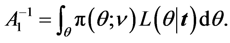 (20)
(20)
The Bayes estimator of a function, say , under squared error and Linex loss functions is given, respectively, by
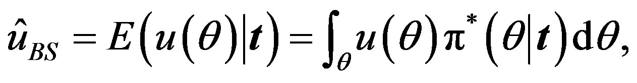 (21)
(21)
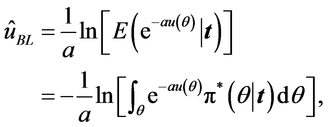 (22)
(22)
where the integral is taken over the five dimensional space and .
.
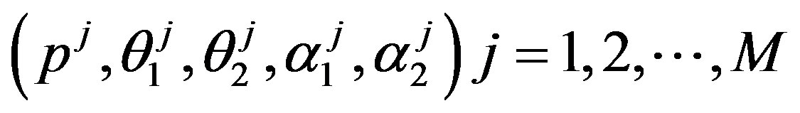
To compute the integral, we can use the Monte Carlo Integration (MCI) method in the form
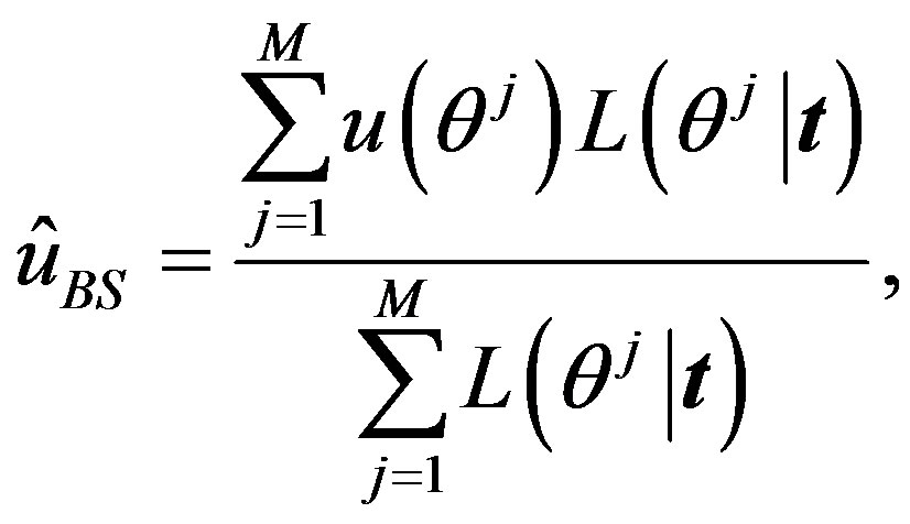 (23)
(23)
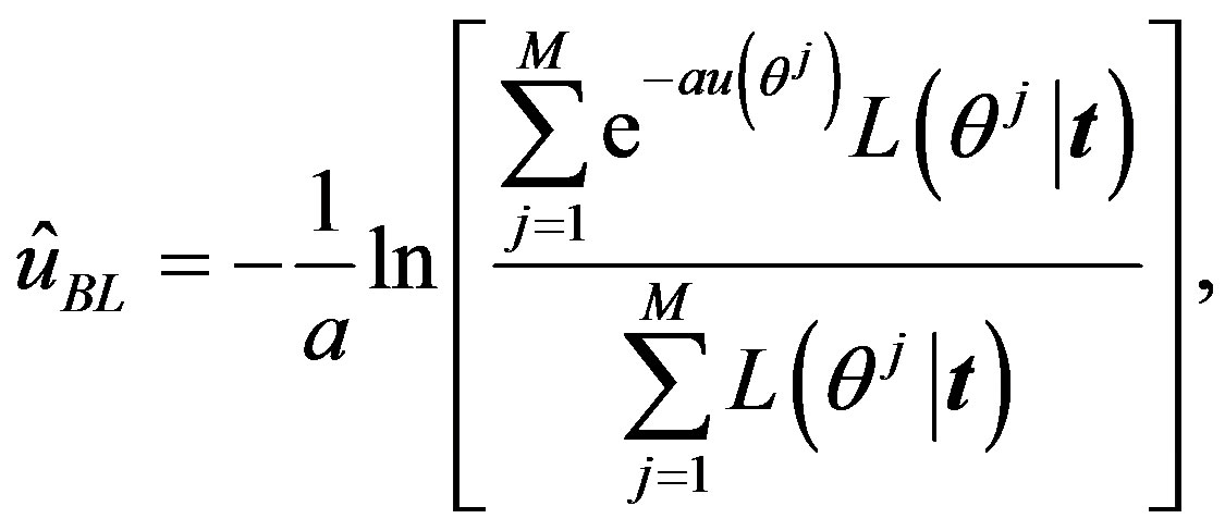 (24)
(24)
where  is generated from the PDF
 , for more details see [30].
Under squared error and Linex loss functions, we can obtain the Bayes estimator of the parameter p, by generating

from the prior (18) and setting  in (23) and (24). The Bayes estimates of
  and
and  can be similarly computed.
3.2. Bayes Estimates When 
The posterior density function can be obtained from (14) and (18), as
 (25)
(25)
where
 (26)
(26)
Under squared error and Linex loss functions, we can obtain the Bayes estimator of the parameter p, by generating
from the prior (18) and setting  in (23) and (24). The Bayes estimates of
  and
and  can be similarly computed.
4. Example
4.1. Gompertz Components
4.1.1. Maximum Likelihood Estimation
Suppose that, for  and
and 
so
 .
.
In this case, the  subpopulation is Gompertz distribution with parameter
For  by substituting
  and
and  in (12), we have the following nonlinear equations
 (27)
(27)
where, for 
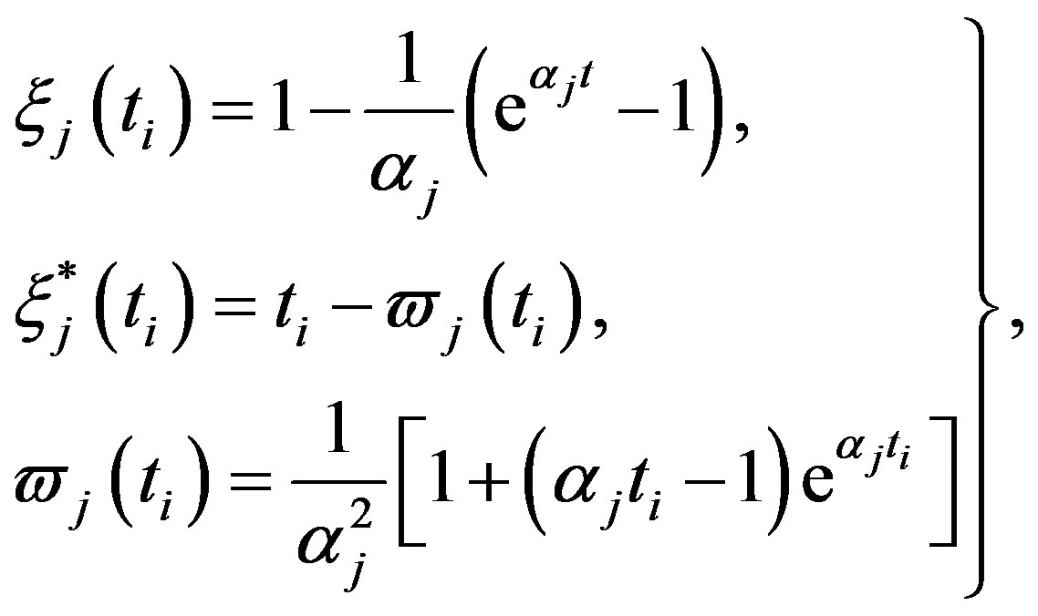 (28)
(28)
 and
and  are the solution of the above nonlinear equations.
Also, for  substituting
  and
and  in (13), (16) and (17), we have the following nonlinear equations:
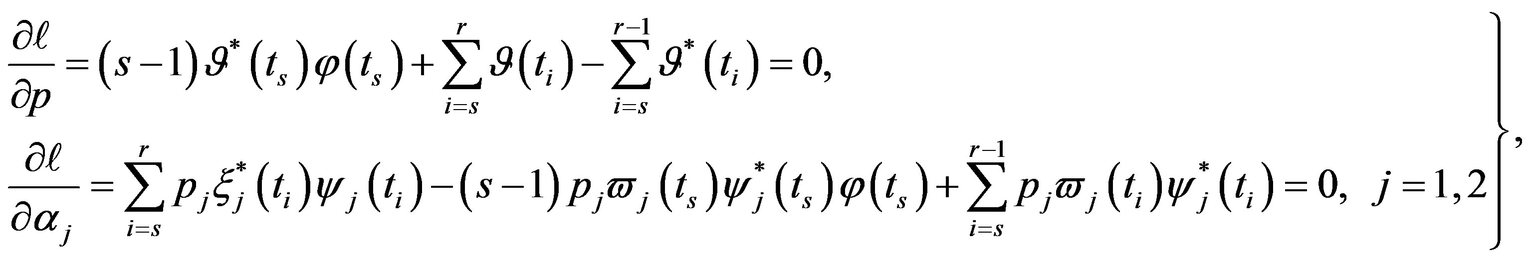
 (29)
(29)
 and
and  are the solution of the above nonlinear equations.
wang#title3_4:spSpecial cases
wang#title3_4:sp1) Upper order statistics
If we put  and
and  in (10),

the likelihood function takes the form
 (30)
(30)
Substituting  and
and  in (27), we have the following nonlinear equations
 (31)
(31)
where .
.
The solution of the nonlinear likelihood equations (31) gives the MLE’s  and
and .
.
wang#title3_4:sp2) Upper record values
If we put  in (14),
  the likelihood function takes the form
 (32)
(32)
Substituting  in (29), we have the following nonlinear equations
 (33)
(33)
The solution of the nonlinear likelihood Equations (33) gives the MLE’s  and
and .
.
4.1.2. Bayes Estimation
Let  and
and  are independent random variables such that
  and for
 ,
,  to follow a left truncated exponential density with parameter
 , as used by [2]. A joint prior density function is then given by
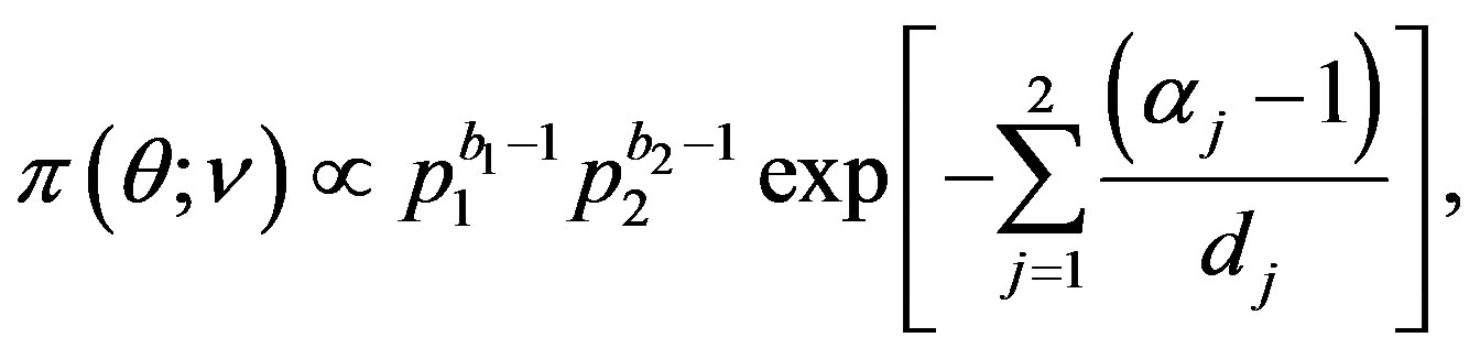 (34)
(34)
where
and 
For  the posterior density function
  then takes the form
 (35)
(35)
For m = −1 the posterior density function then takes the form
 (36)
(36)
Under squared error and Linex loss functions, we can obtain the Bayes estimator of the parameter  by generating
  from the prior (34) and setting
  in (23) and (24). The Bayes estimates of
  and
and  can be similarly computed.
wang#title3_4:spSpecial cases
wang#title3_4:sp1) Upper order statistics
If we put  and
and  in (35),
  the posterior density function takes the form
 (37)
(37)
wang#title3_4:sp2) Upper record values
If we put  in (36),
  the posterior density function takes the form
 (38)
(38)
Under squared error and Linex loss functions, we can obtain the Bayes estimator of the parameter  by generating
  from the prior (34) and setting
  in (23) and (24). The Bayes estimates of
  and
and  can be similarly computed.
5. Simulation Study
A comparison between ML and Bayes estimators, under either a squared error or a Linex loss functions, is made using a Monte Carlo simulation study in the two cases upper order statistics and upper record values according to the following steps:
1) For a given values of the prior parameters  generate a random value
  from the
  distribution.
2) For a given values of the prior parameters  for
for  generate a random value
  from the
  distribution.
3) Using the generated values of  and
and  we generate a random sample of size
  from a mixture of two
  components,
  as follows:
• generate two observations  from
from 
• if  then
then

otherwise
• 
• repeat above steps  times to get a sample of size
 .
.
4) The sample obtained in Step 3 is ordered.
5) The MLE’s of the parameters  and
and  are obtained by solving the nonlinear Equations (31), by using Mathematica 6.
6) Using the generated values of  and
and  we generate upper record values of size
  from a mixture of two
  components.
7) The MLE’s of the parameters  and
and  are obtained by solving the nonlinear Equations (33), by using Mathematica 6.
8) The Bayes estimates under squared error and Linex loss functions (BES, BEL), of  and
and  are computed, by using MCI forms (23) and (24), respectively.
9) The squared deviations  are computed for different samples and censoring sizes, where
  stands for the parameter and
  its estimate (ML or Bayes).
10) The above Steps (3)-(9) are repeated 1000 times. The averages and the estimated risks (ER) are computed over the 1000 repetitions by averaging the estimates and the squared deviations, respectively.
The computational (our) results were computed by using Mathematica 6.0. In all above cases the prior parameters chosen as
 , which yield the generated values of
 and
and  (as the true values). The true values of
  and
and  when
when , are computed to be
  and
and 
 The value of the shape parameter
  of the Linex loss function is
 . The averages and the estimated risks (ER) are displayed in Tables 1-4. Figures 1 and 2 represent the estimated risks of the estimates in the case of upper order statistics. Figures 3 and 4 represent the estimated risks of the estimates
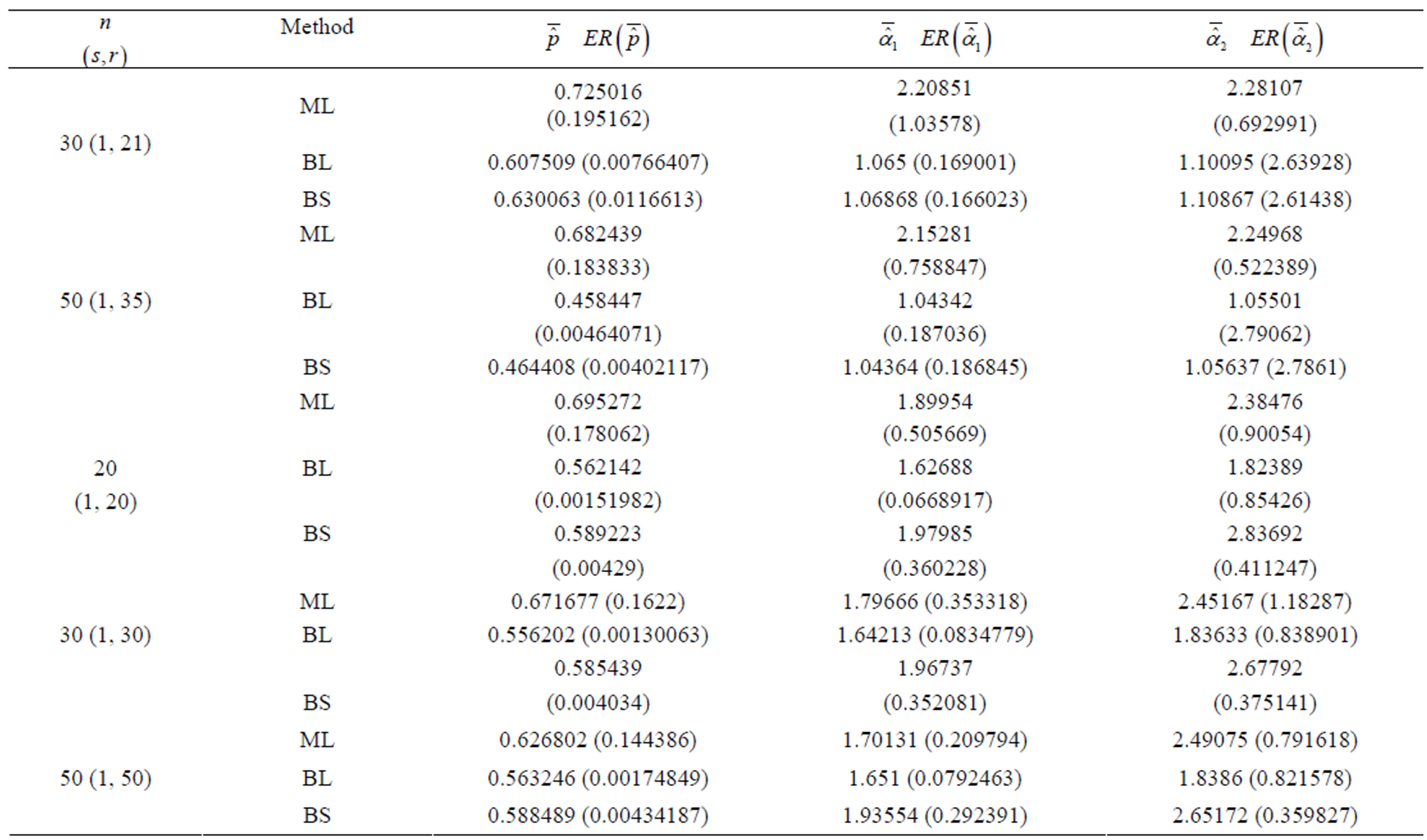
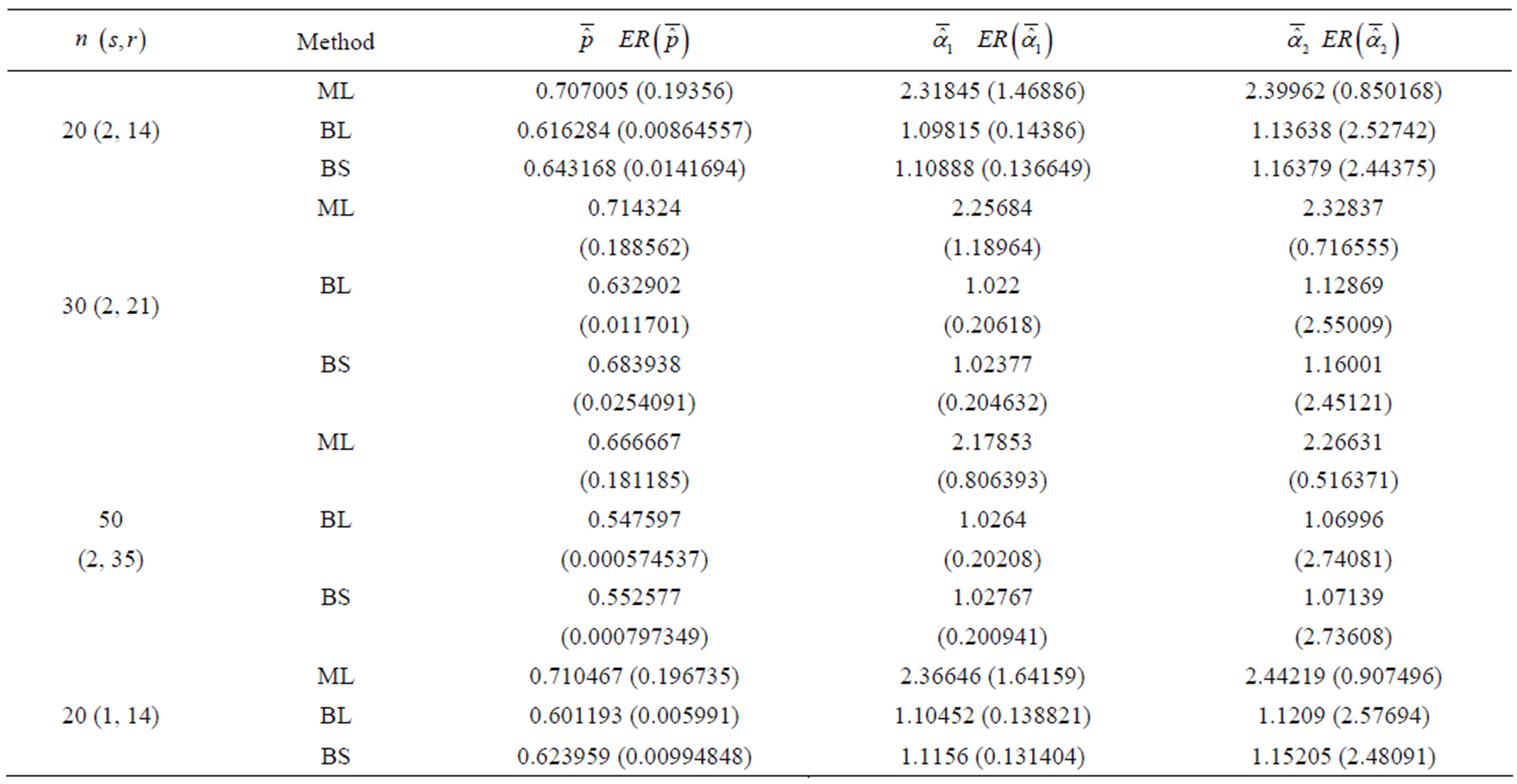
Table 1. (Upper order statistics) Averages and Estimated Risks (ER) of the estimates of  for different samples and censoring sizes.
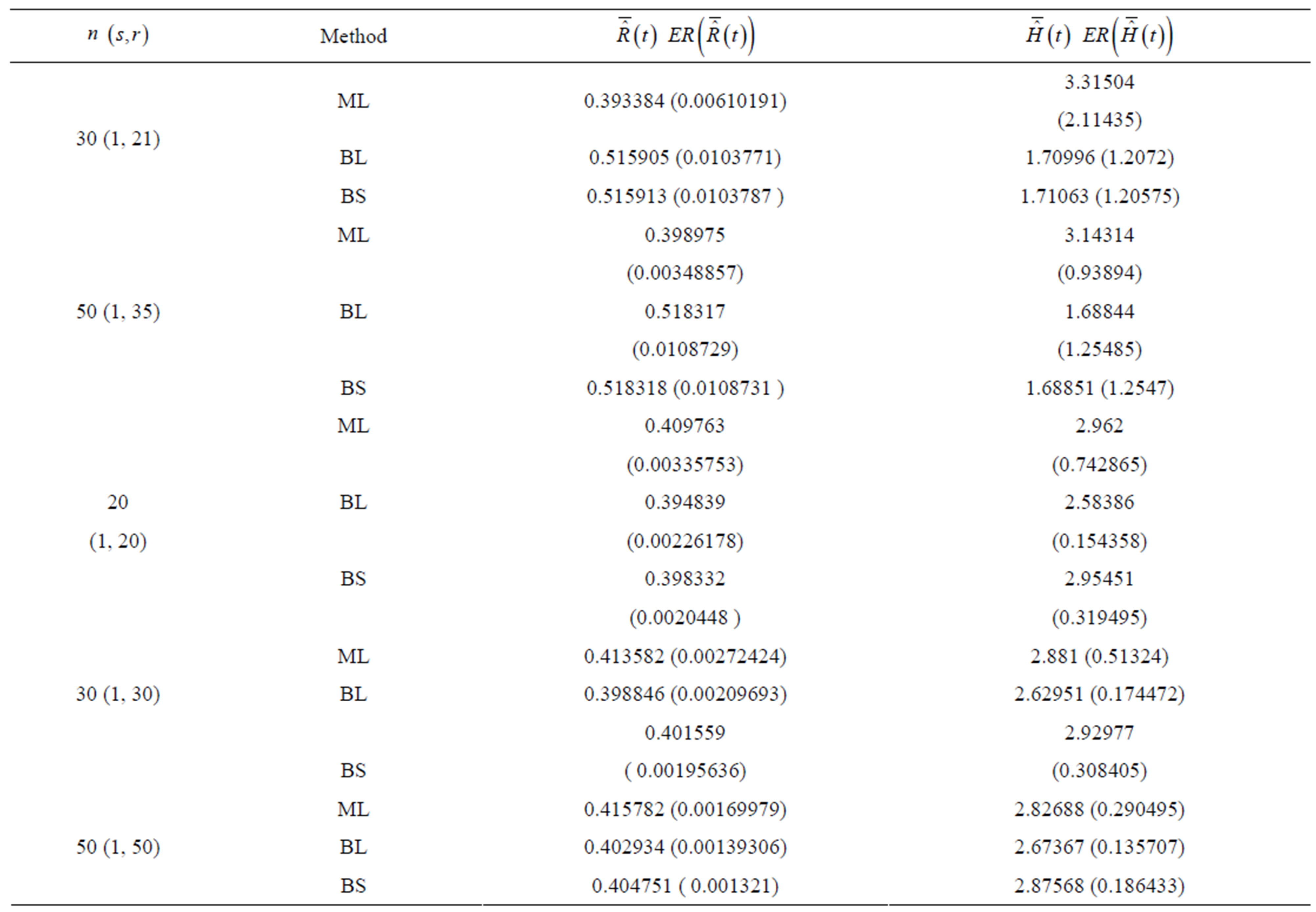
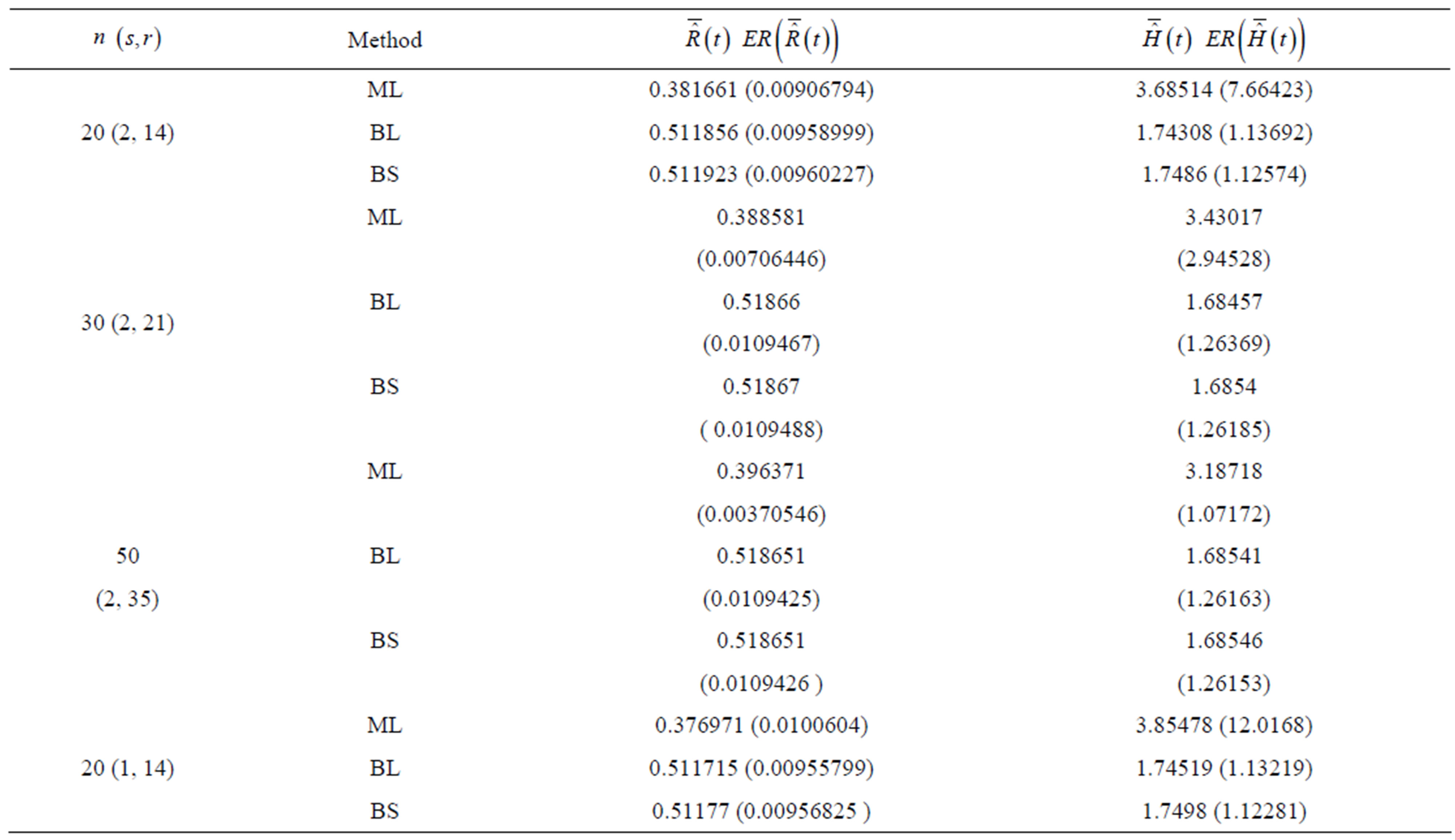
Table 2. (Upper order statistics) averages and estimated risks (ER) of the estimates of  and
and  for different sample and censoring sizes.
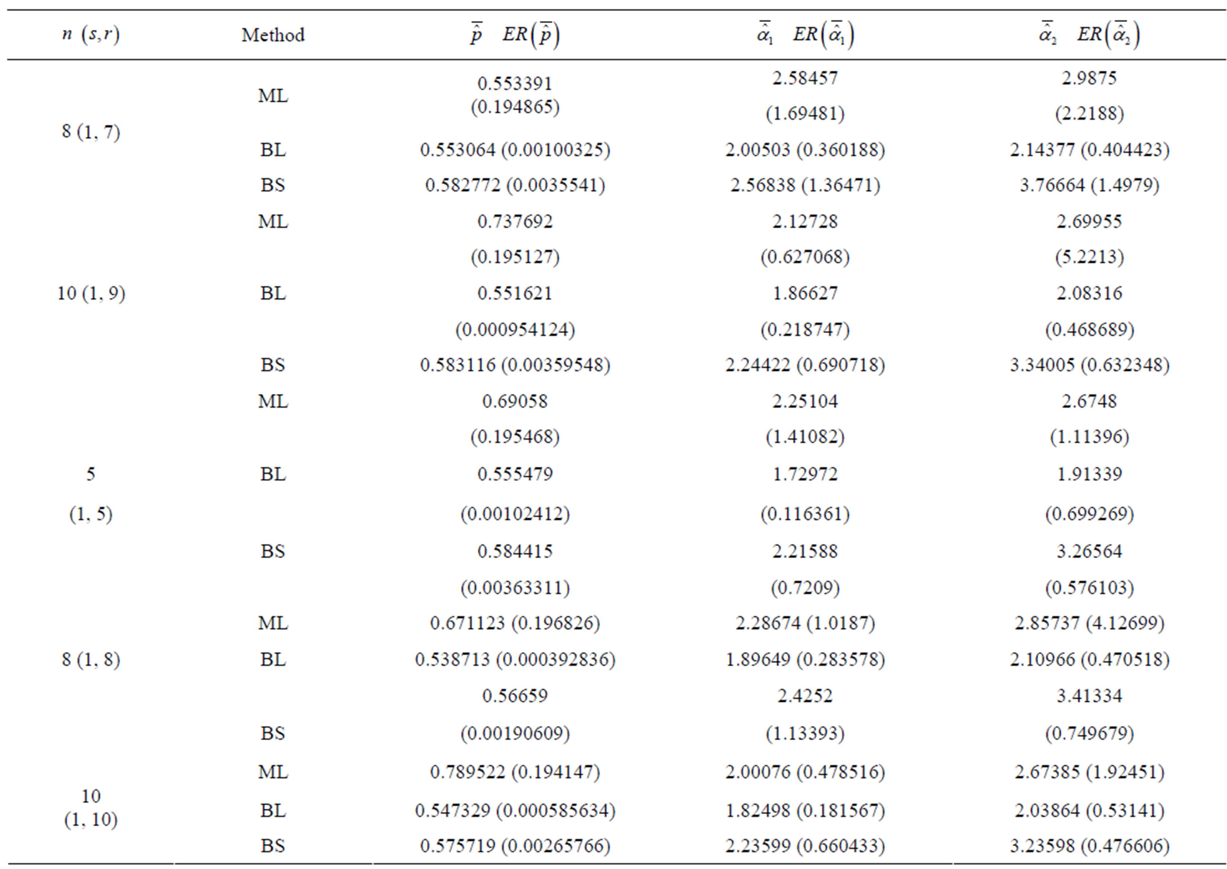
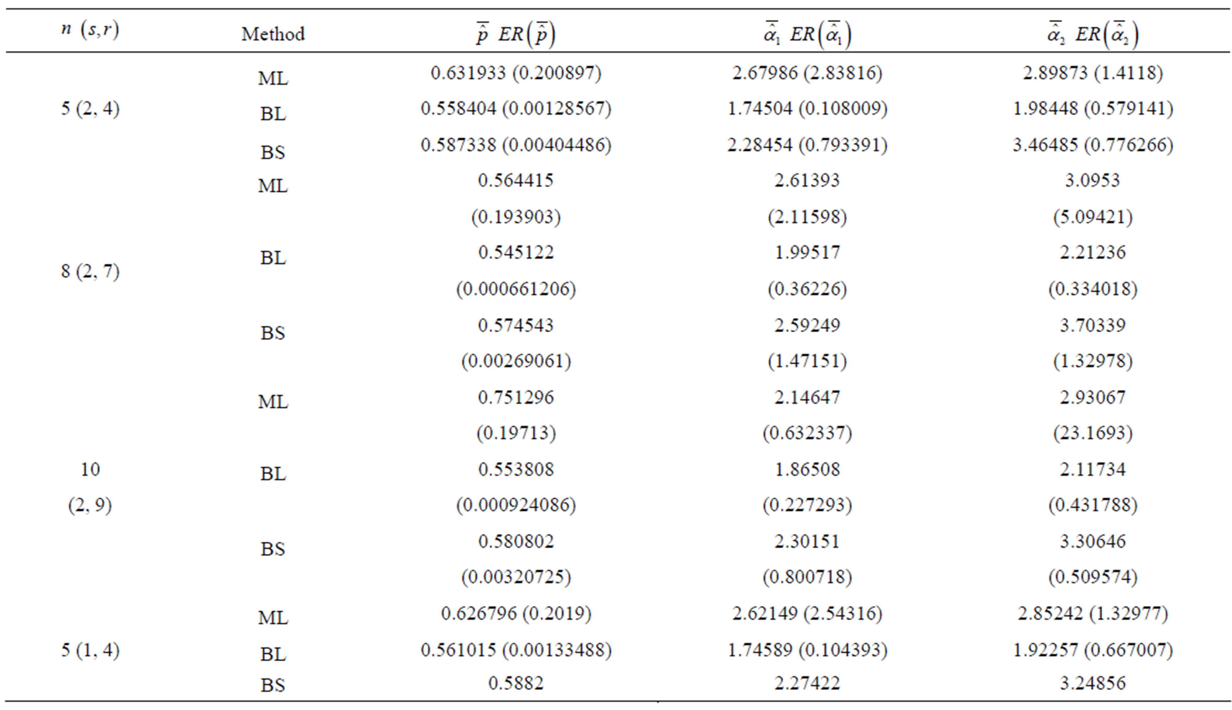
Table 3. (Upper record values) Averages and Estimated Risks (ER) of the estimates of  for different sample
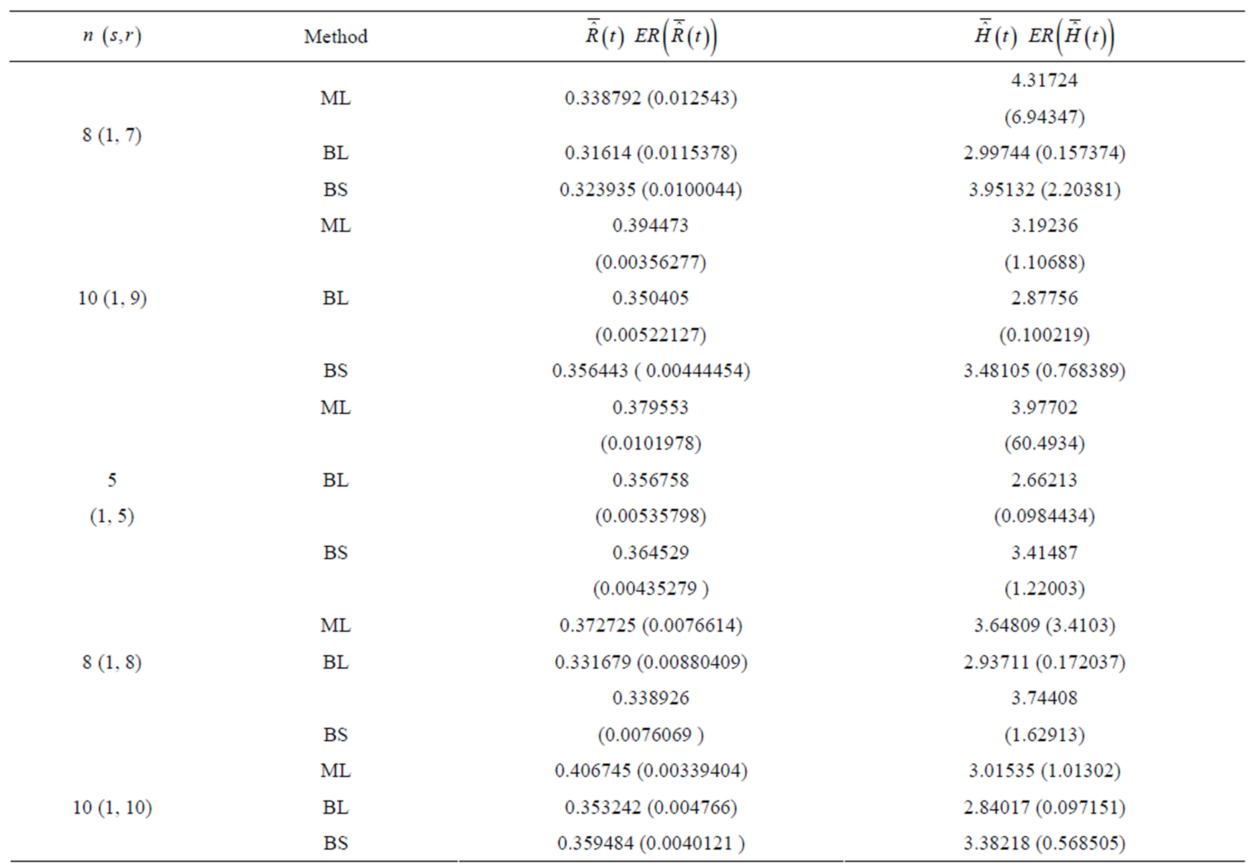
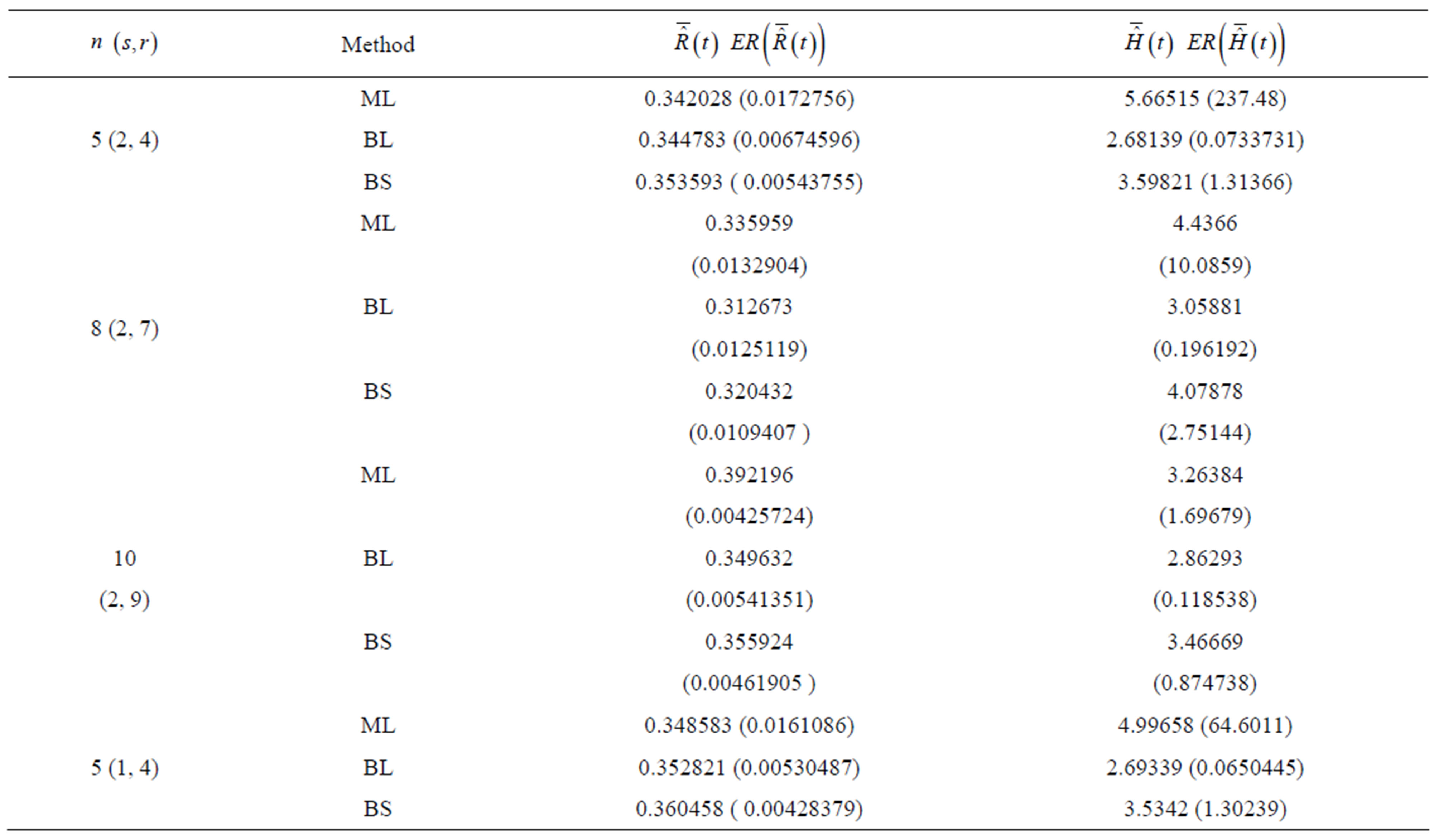
Table 4. (Upper record values) Averages and Estimated Risks (ER) of the estimates of  and
and  for different sample and censoring sizes.
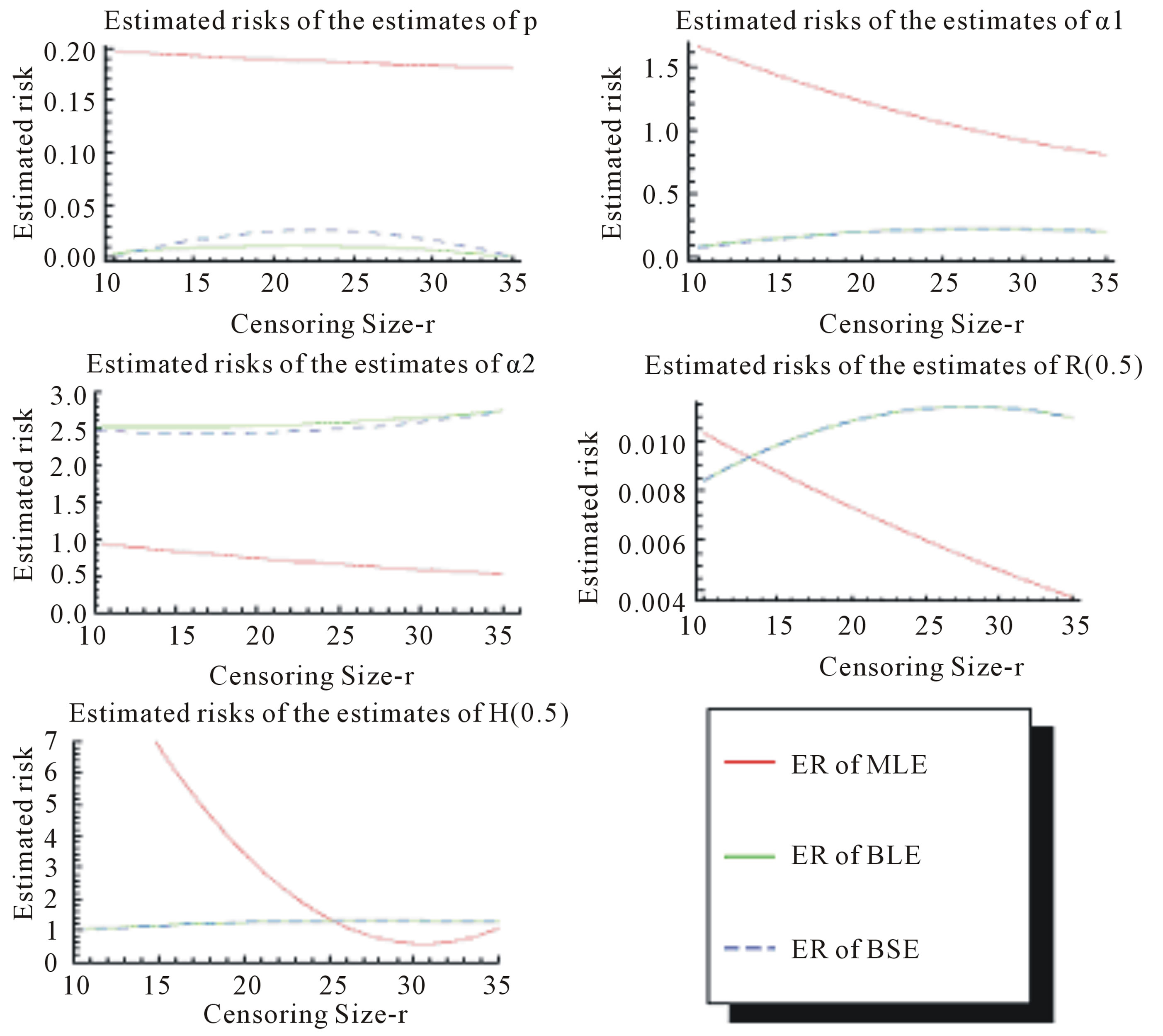
Figure 1. Estimated Risks (ER) of the estimates of ,
,  and
and  based on doubly Type II censored samples (s = 2).
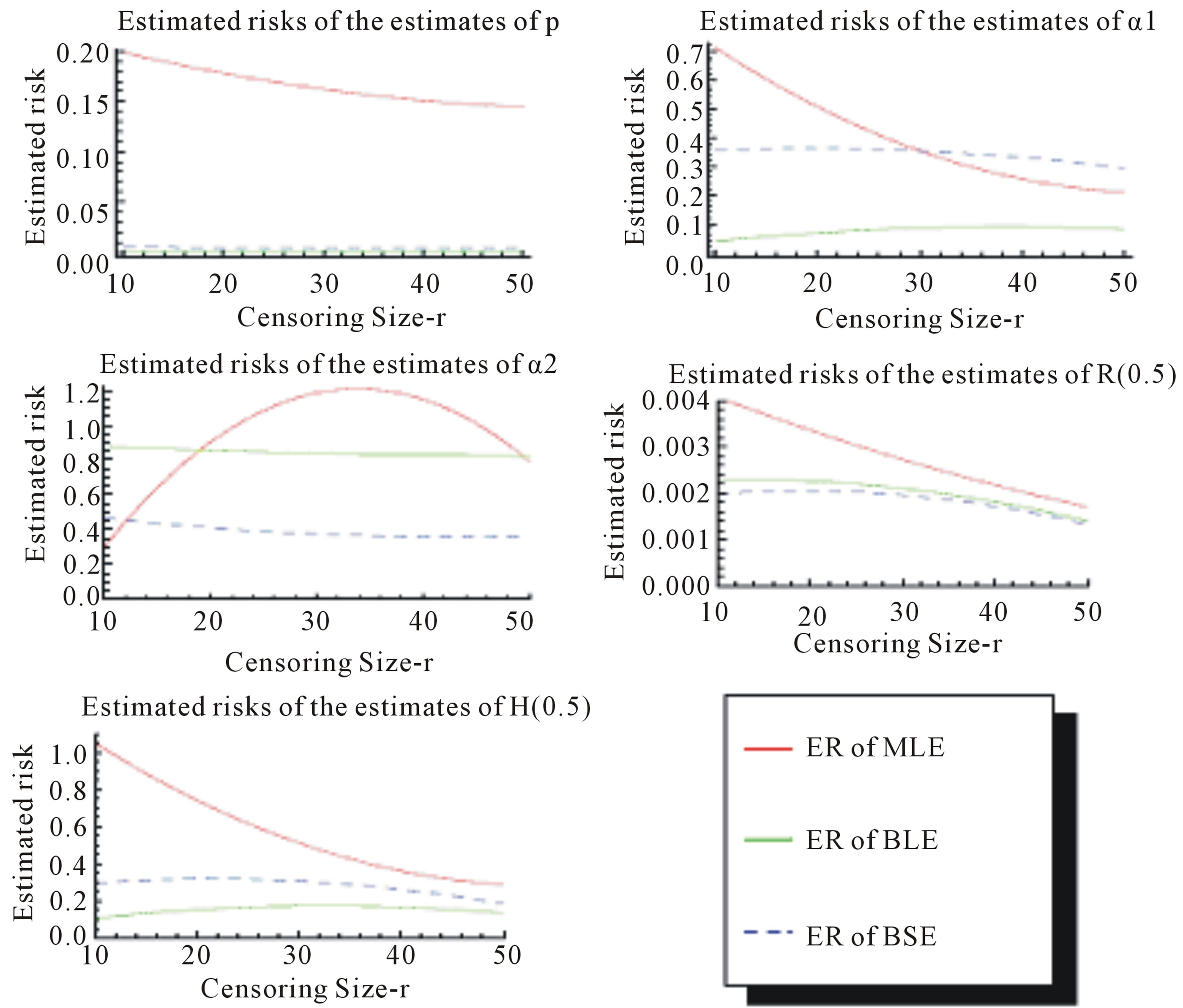
Figure 2. Estimated Risks (ER) of the estimates of ,
,  and
and  complete samples.
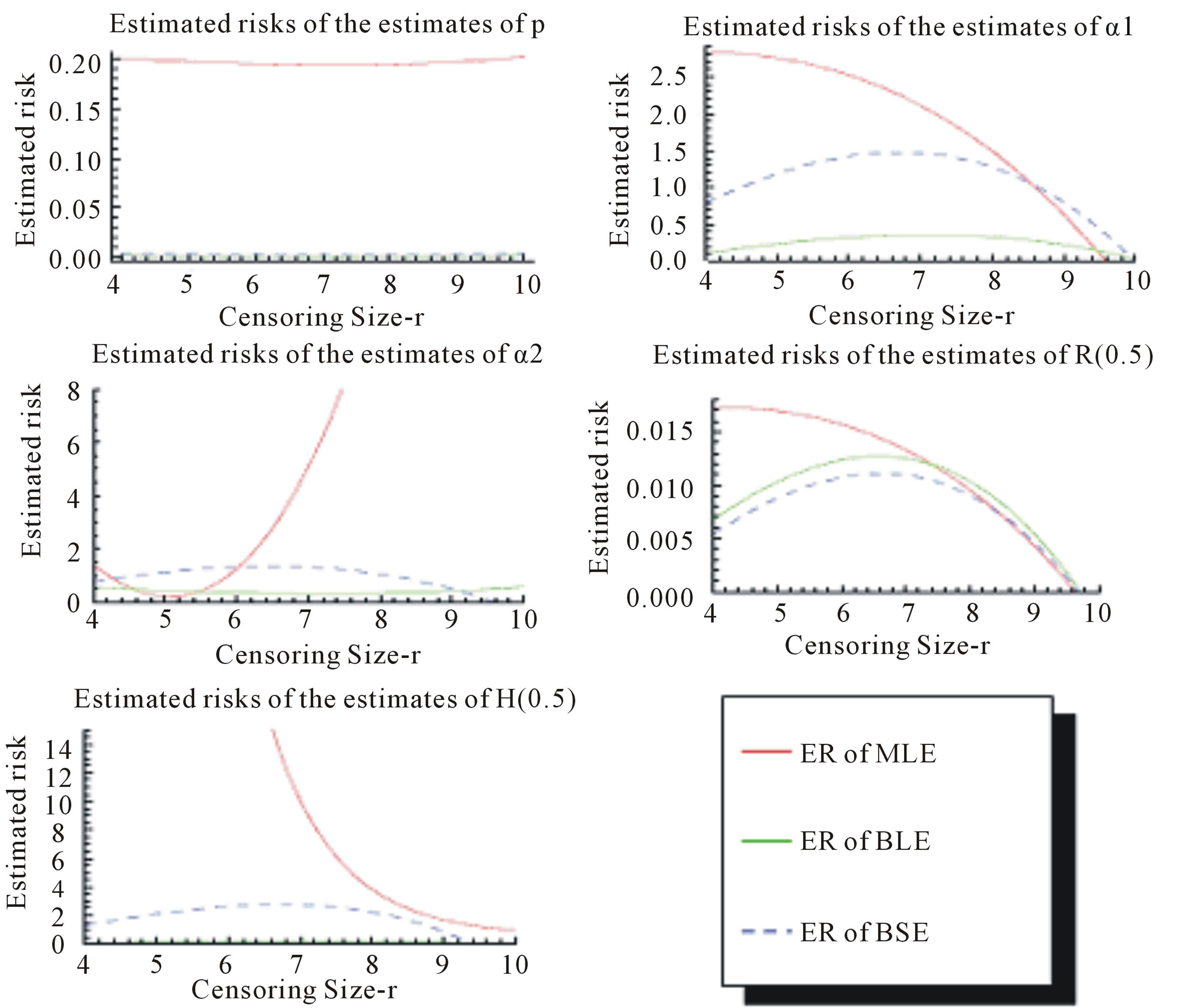
Figure 3. Estimated Risks (ER) of the estimates of ,
,  and
and  based on doubly Type II censored samples (s = 2).
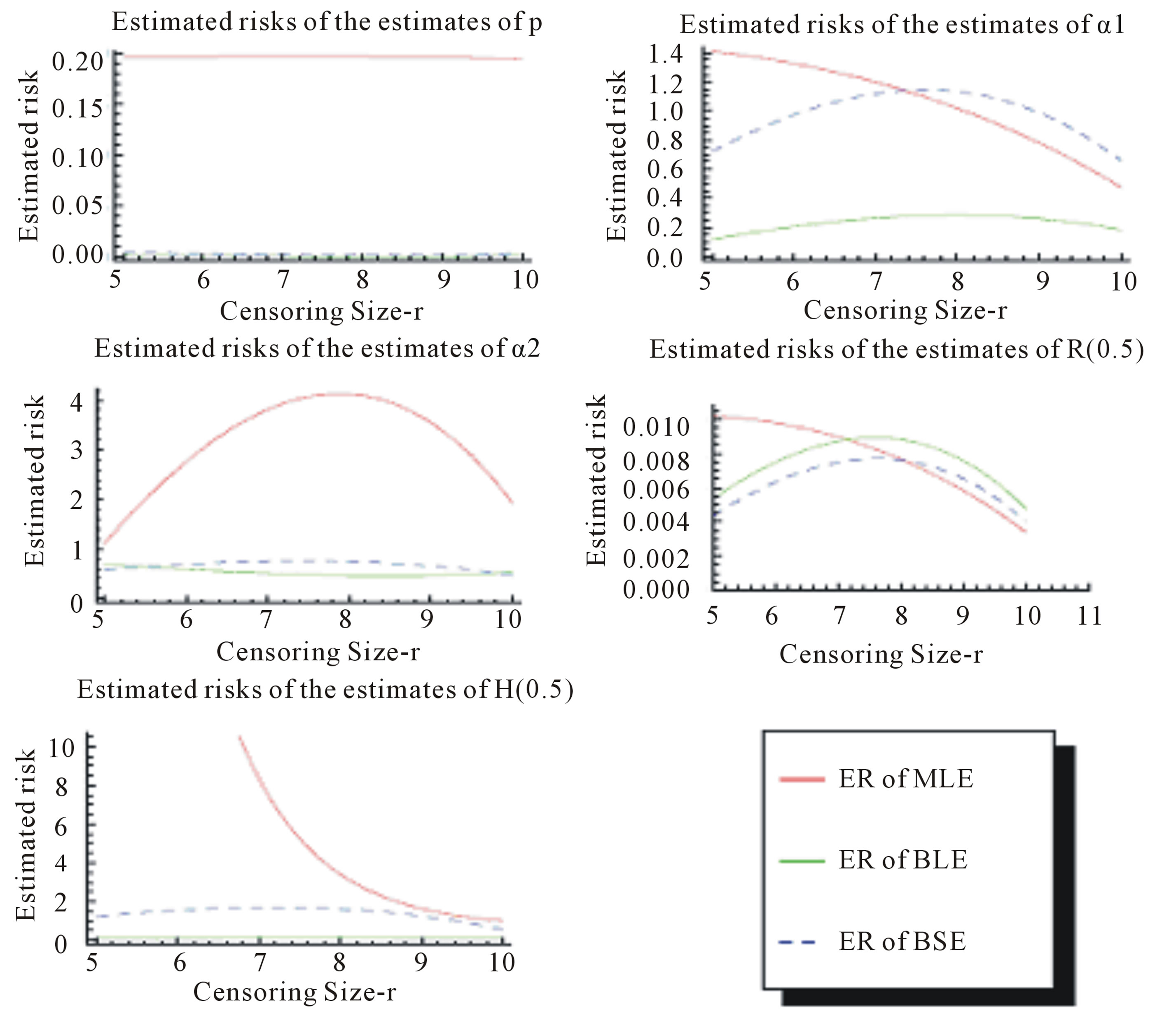
Figure 4. Estimated Risks (ER) of the estimates of ,
,  and
and  complete samples.
in the case of upper record values.
6 Concluding Remarks
1) Estimation of the parameters of the finite mixture model of two Gompertz distributions are considered from a Bayesian approach based on gos’s. A compareson between ML and Bayes estimators, under either a squared error loss or a Linex loss, is made by using a Monte Carlo simulation study in both two cases considering order statistics and upper record values cases.
2) From Tables 1 and 2, we see that in most of the considered cases, the ER’s of the estimates decrease as n increases. In complete sample case, the Bayes estimates of p,  and HRF under Linex loss function have the smallest ER’s as compared with their corresponding estimates under squared error loss function or MLE’, while the ER’s of the Bayes estimates of
  and RF under squared error loss functions are the smallest estimated risks. For censored samples, the Bayes estimates of p under Linex loss function have the smallest ER’s as compared with their corresponding estimates under squared error loss function or MLE’s. While, the Bayes estimates (against the proposed prior) of
  and HRF under squared error loss function have the smallest ER’s as compared with their corresponding estimates. It is observed that MLE’s for HRF perform best when sample size n is increased. Also, we note that the MLE’s of
  and RF have the smallest ER’s as compared with Bayes estimates.
3) From Tables 3 and 4, we see that the Bayes estimates (against the proposed prior) of the parameters and HRF under Linex loss function have the smallest ER's as compared with their corresponding estimates under squared error loss function or MLE’s. While, the Bayes estimates of  (for complete sample) and RF under squared error loss function have the smallest ER’s as compared with both Bayes estimates under Linex loss function or the MLE’s. Also, it is observed that MLE's for RF perform best when sample size n is increased.
4) If the mixing proportion p is known, [2] estimated the parameters  reliability and hazard rate functions based on Types I and II censored samples.
REFERENCES
- A. S. Papadapoulos and W. J. Padgett, “On Bayes Estimation for Mixtures of Two Exponential-Life-Distributions from Right-Censored Samples,” IEEE Transactions on Reliability, Vol. 35, No. 1, 1986, pp. 102-105. doi:10.1109/TR.1986.4335364
- E. K. AL-Hussaini, G. R. Al-Dayian and S. A. Adham, “On Finite Mixture of Two-Component Gompertz Lifetime Model,” Journal of Statistical Computation and Simulation, Vol. 67, No. 1, 2000, pp. 1-20.
- E. K. AL-Hussaini and S. F. Ateya, “Bayes Estimations under a Mixture of Truncated Type I Generalized Logistic Components Model,” Journal of Applied Statistical Science, Vol. 4 No. 2, 2005, pp. 183-208.
- Z. F. Jaheen, “On Record Statistics from a Mixture of Two Exponential Distributions,” Journal of Statistical Computation and Simulation, Vol. 75, No. 1, 2005, pp. 1- 11. doi:10.1080/00949650410001646924
- E. K. AL-Hussaini and R. A. AL-Jarallah, “Bayes Inference under a Finite Mixture of Two Compound Gompertz Components Model,” Cairo University, 2006.
- K. S. Sultan, M. A. Ismail and A. S. Al-Moisheer, “Mixture of Two Inverse Weibull Distributions: Properties and Estimation,” Computational Statistics & Data Analysis, Vol. 51, No. 11, 2007, pp. 5377-5387. doi:10.1016/j.csda.2006.09.016
- U. Kamps, “A Concept of Generalized Order Statistics,” Journal of Statistical Planning and Inference, Vol. 48, No. 1, 1995, pp. 1-23. doi:10.1016/0378-3758(94)00147-N
- M. Ahsanullah, “Generalized Order Statistics from Two Parameter Uniform Distribution,” Communications in Statistics—Theory and Methods, Vol. 25, No. 10, 1996, pp. 2311-2318. doi:10.1080/03610929608831840
- U. Kamps and U. Gather, “Characteristic Property of Generalized Order Statistics for Exponential Distributions,” Applied Mathematics (Warsaw), Vol. 24, No. 4, 1997, pp. 383-391.
- E. Cramer and U. Kamps, “Relations for Expectations of Functions of Generalized Order Statistics,” Journal of Statistical Planning and Inference, Vol. 89, No. 1-2, 2000, pp. 79-89. doi:10.1016/S0378-3758(00)00074-4
- M. Habibullah and M. Ahsanullah, “Estimation of Parameters of a Pareto Distribution by Generalized Order Statistics,” Communications in Statistics—Theory and Methods, Vol. 29, No. 7, 2000, pp. 1597-1609. doi:10.1080/03610920008832567
- E. K. AL-Hussaini and A. A. Ahmad, “On Bayesian Predictive Distributions of Generalized Order Statistics,” Metrika, Vol. 57, No. 2, 2003, pp. 165-176. doi:10.1007/s001840200207
- E. K. AL-Hussaini, “Generalized Order Statistics: Prospective and Applications,” Journal of Applied Statistical Science, Vol. 13, No. 1, 2004, pp. 59-85.
- Z. F. Jaheen, “On Bayesian Prediction of Generalized Order Statistics,” Journal of Applied Statistical Science, Vol. 1, No. 3, 2002, pp.191-204.
- Z. F. Jaheen, “Estimation Based on Generalized Order Statistics from the Burr Model,” Communications in Statistics—Theory and Methods, Vol. 34, No. 4, 2005, pp. 785-794. doi:10.1081/STA-200054408
- A. A. Ahmad, “Relations for Single and Product Moments of Generalized Order Statistics from Doubly Truncated Burr Type XII Distribution,” Journal of the Egyptian Mathematical Society, Vol. 15, No. , 2007, pp. 117- 128.
- A. A. Ahmad, “Single and product Moments of Generalized order Statistics from Linear Exponential Distribution,” Communications in Statistics—Theory and Methods, Vol. 37, No. 8, 2008, pp. 1162- 1172. doi:10.1080/03610920701713344
- S. F. Ateya and A. A. Ahmad, “Inferences Based on Generalized Order Statistics under Truncated Type I generalized Logistic Distribution,” Statistics, Vol. 45, No. 4, 2011, pp. 389-402. doi:10.1080/02331881003650149
- T. A. Abu-Shal and A. M. AL-Zaydi, “Estimation Based on Generalized Order Statistics from a Mixture of Two Rayleigh Distributions,” International Journal of Statistics and Probability, Vol. 1, No. 2, 2012, pp. 79-90.
- T. A. Abu-Shal and A. M. AL-Zaydi, “Prediction Based on Generalized Order Statistics from a Mixture of Rayleigh Distributions Using MCMC Algorithm,” Open Journal of Statistics, Vol. 2, No. 3, 2012, pp. 356-367. doi:10.4236/ojs.2012.23044
- B. S. Everitt and D. J. Hand, “Finite Mixture Distributions,” University Press, Cambridge, 1981. doi:10.1007/978-94-009-5897-5
- D. M. Titterington, A. F. M. Smith and U. E. Makov, “Statistical Analysis of Finite Mixture Distributions,” John Wiley and Sons, New York, 1985.
- G. J. McLachlan and K. E. Basford, “Mixture Models: Inferences and Applications to Clustering,” Marcel Dekker, New York, 1988.
- H. Teicher, “Identifiability of Finite Mixtures,” The Annals of Mathematical Statistics, Vol. 34, No. 4, 1963, pp. 1265-1269. doi:10.1214/aoms/1177703862
- E. K. AL-Hussaini and K. E. Ahmad, “On the Identifiability of Finite Mixtures of Distributions,” Transactions on Information Theory, Vol. 27, No. 5, 1981, pp. 664- 668.
- K. E. Ahmad, “Identifiability of Finite Mixtures Using a New Transform,” The Annals of Mathematical Statistics, Vol. 40, No. 2, 1988, pp. 261-265. doi:10.1007/BF00052342
- A. A. Ahmad, “On Bayesian Interval Prediction of Future Generalized Order Statistics Using Doubly Censoring,” Statistics, Vol. 45, No. 5, 2011, pp. 413- 425. doi:10.1080/02331881003650123
- U. Kamps, “A Concept of Generalized Order Statistics,” Journal of Statistical Planning and Inference, Vol. 48, No. 1, 1995, pp. 1-23. doi:10.1016/0378-3758(94)00147-N
- E. K. AL-Hussaini, “Prediction, Observables from a General Class of Distributions,” Journal of Statistical Planning and Inference, Vol. 79, No. 1, 1999, pp. 79-91. doi:10.1016/S0378-3758(98)00228-6
- S. J. Press, “Subjective and Objective Bayesian Statistics: Principles, Models and Applications,” Wiley, New York, 2003.