Open Journal of Geology
Vol.3 No.5(2013), Article ID:36620,9 pages DOI:10.4236/ojg.2013.35040
Methodology and Equations of Mineral Production Forecast
—Part I. Crude Oil in the UK and Gold in Nevada, USA. Prediction of wang#:br Late Stages of Production
PETROINVESTENERGY, Houston, USA
Email: sperez@petroinvestenergy.com
Copyright © 2013 Sergio Pérez Rodríguez. This is an open access article distributed under the Creative Commons Attribution License, which permits unrestricted use, distribution, and reproduction in any medium, provided the original work is properly cited.
Received June 29, 2013; revised July 29, 2013; accepted August 10, 2013
Keywords: mineral; mining; oil; gas; montecarlo simulation
ABSTRACT
The equations of mineral production forecast link the change in time of mineral reserves with the production and the ratio of reserves to production. These equations allow us to model the development of the mineral resources evaluated at any scale. Probabilistic bidimensional charts made from montecarlo simulations provide intervals of confidence for the forecasts. The set of equations is devised and presented for a variety of applications to the oil and gas industry, as well to the production of any other mineral resource, either metals or non metals, whose ore deposit volumes and production might be quantified. The cases studied in the UK and USA are at late stages of production, periods for what the equations are most suitable to be applied without further adjustments. Experimental design allows the diagnosis of the likely values of the variables pertaining to the equations, in order to achieve the results provided by conventional production forecasts or to explore other scenarios of investigation. The method can be practical to evaluate commitments of production of mineral resources with time, to support strategic plans for companies, corporations, countries or regions based on those evaluations, for the screening and ranking of mineral assets based on their production potential and many other tasks where the prediction of future volumes of mineral production is required.
1. Introduction
In the oil and gas industry, as well as in other areas of mineral development, one of the most difficult tasks is to make a confident time production forecast. Working with one or few oil and gas reservoirs, the traditional use of decline curves, of mass balance and even simulations is often enough to deal with the matter. Nevertheless, when many oil and gas reservoirs are considered altogether, to handle the cumulative output of the variety of decline curves or simulations is cumbersome, if not unpractical. Options to tackle these challenges are usually based on trend analysis of decline rates, which rely on methods of extrapolation from historical datasets. We shall see the comparison of the results from the equations and familiar predictions based on this kind of conventional forecasts. A latter study will be left the contrast with the most sophisticated approach to model production of commodities given by the Hubbert’s linearization and the logistic curve [1], which deserves a technical article of its own.
Keeping the distances, similar situation happens when it is requested an appraisal of the future production of minerals, like gold, silver, or any other resource, strategic or not. We shall see the equations of mineral production forecast (EMPF) and a general technique that is applicable even for these latter cases, where solid materials but not fluids or gases are extracted from mineral reservoirs.
The structure of the article follows the next sequence of steps:
Conceptualization and formulation of the equations of mineral production forecast (EMPF) and a methodology to apply them in practical cases.
Presentation and application of the methodology and equations to the analysis of study cases where it is noticeable that embraces a universal range of applications and scales of mineral production.
In the latter step, we also pursue the following objectives:
To compare results of conventional and EMPF based forecasts.
To provide the likely dimension of the variables involved in the equations of MPF to achieve the production commitments based on conventional forecasts. This task is accomplished via experimental design.
To diagnose, under the light of EMPF and the statistical record of the variables, how feasible the production commitments based on conventional forecasts are.
2. Presentation of the Equations of Mineral Production Forecast (EMPF)
The concept of production reserves ratio (PRR) is a useful reference to evaluate the extent and rate of reserves development. It provides a quick point of reference about how fast the reserves are developed and hence how long they will be available. The expression of the PRR usually is assumed as a percentage (Production/Reserves x 100).
To enhance mathematical operations, the expression used for the PRR in the next developments is the fractional way, what is understood as the division of Production between Reserves, So PRR = Production/Reserves.
For the sake of further developments, the variables are considered as following:
Production-reserves ratio (PRR) for every year is defined as the respective production of that year divided by the reserves available at the beginning of the year. In the equations it will be designated with a capital C.
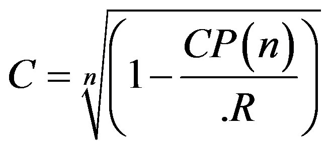
To link production (P) and reserves (R), its ratios and volumes, in a mathematical way, the following equations are proposed (See Annex 1. for the demonstration of Eq. 1 via mathematical induction):
• The amount of reserves available at every year R(n) assumes the expression of a Geometric Sequence, where each term is the result of the multiplication of the previous one by the arithmetic complement of the production-reserves ratio (C). The Reserves then takes a mathematical form that is in direct proportion of the initial reserves R0 and a power function of the arithmetic complement of C.
 (1)
(1)
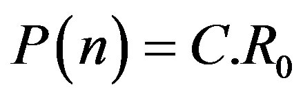
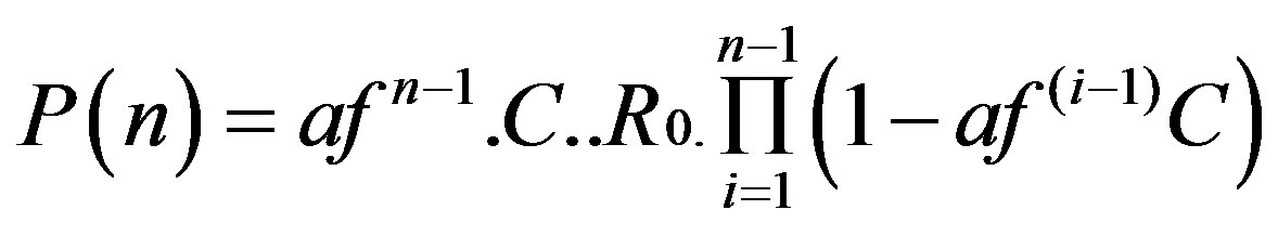
• The total production at any year P(n) is proportional to a power function of the arithmetic complement of the production-reserves ratio (C), and also in direct proportion to the product of C times the initial reserves R0. The sequence of successive production volumes at every year is regarded as a geometrical sequence.
Due to its direct connection with production as a dependant variable, Equation (2) is regarded as a fundamental one of the set. It will be applied to make the production forecasts of the cases under study:
 (2)
(2)
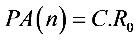
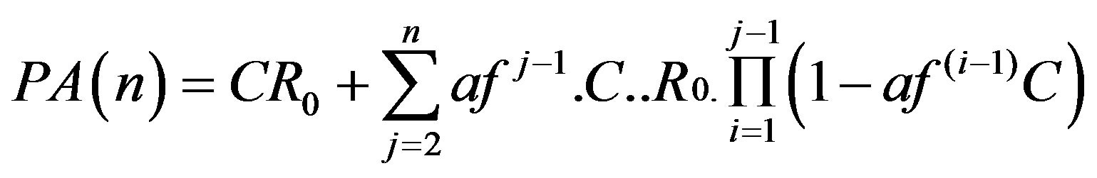
• The cumulative production for a given year PA(n) takes the mathematical expression of a geometric series. A straightforward algebraic transformation leads to the calculation of the cumulative production as a polynomial function of the PRR. This polynomial equals the addition of the production at every year, being considered as terms of a geometrical sequence.
 (3)
(3)
• Lets consider remaining reserves as a fraction (XR, 1 ≥ XR > 0) of the initial reserves. Then, the amount of years (n) needed to reach some remaining reserves (XR) is inversely proportional to the logarithm of the arithmetic complement of C and directly proportional to the logarithm of XR. Given a fixed C, this implies the calculation of the final year of production for the total depletion of reserves (XR near zero) from the logarithm of C.
 (4)
(4)
This Equation leads to a graphical solution (Figure 1) of the question how much time does it takes to achieve the production of a determined fraction of reserves?
So, to get the amount of years to produce a fraction of reserves (1-XR) is enough to estimate n for XR (see Figure 1). Given a predetermined production reserve ratio (0.1 ≤ C ≤ 0.9) the fraction of remaining reserves XR, and also the fraction of reserves produced (1-XR) are obtained from Equation (4).
Differential calculus could be used to estimate the rate of change in reservoir volumes, production and cumulative production.
The rate of change of the reserves (DR(n)), production (DP(n)) and the cumulative production (DPA(n))with time would be, from equations (1), (2) and (3):
 (5)
(5)
 (6)
(6)
 (7)
(7)
Obviously, the rate of change of the reserves is equal to the one of the cumulative production (DR(n) = DPA(n)). Also it is noticed the equations require to consider at least two years in advance to be applied.
For practical purposes, the rate of change of these variables could be used to try several scenarios and to evaluate most favorable production rates, as a help to analyze and manage reserves, and in general, to have basis to support optimal decisions in this field.
3. Methodology and Results
The procedure to determine the outcome of the forecast,
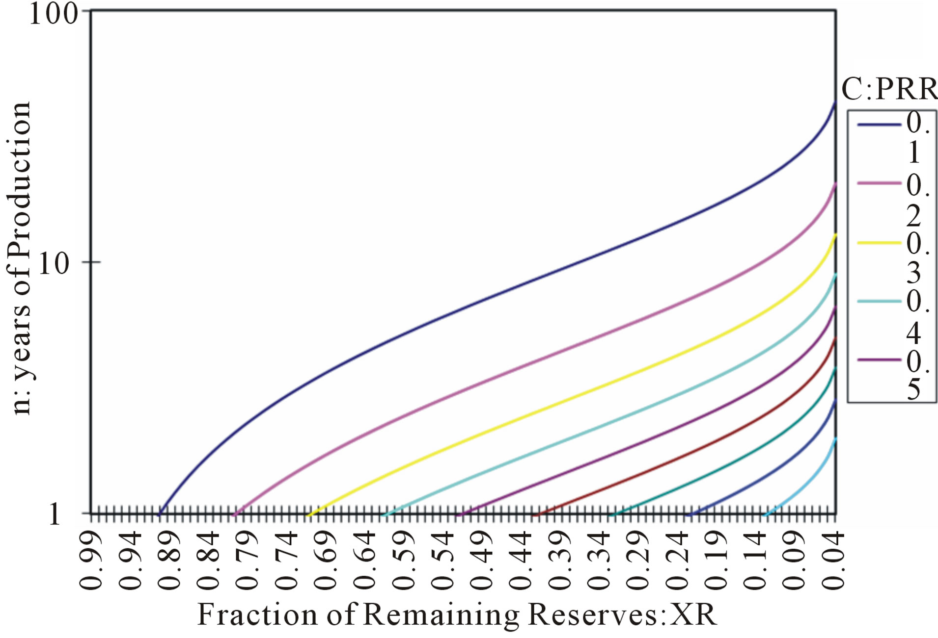
Figure 1. Graphical display of the depletion of reserves (fixed PRR).
including the use of the montecarlo simulation is as follows:
1) From the original data of Reserves and Production work out the Production Reserves Ratio 2) Make trend analysis and identify best fitted functions for the data of Reserves, Production and Production Reserves Ratio.
3) Determine an initial forecast of production using the function that best fits the trend for this parameter. Use the function that models the reserves to appraise its value for the last or current year if it is only available the production for that year.
4) For the Reserves and the Production Reserves Ratio calculate the following descriptive statistical parameters: mean or average, standard deviation, and variance.
5) Estimate the Coefficient of Variation of the Reserves and of the Production Reserves Ratio. This Coefficient will be used to estimate the Standard Deviation of the variables during the simulation.
6) Distributions are fitted and assigned to the Reserves and PRR using as a reference the statistical data available.
If many distributions display the same goodness of fit, to select the most appropriate one it is followed the criteria of the lowest coefficient of variation [2]. In the first case under study, Normal Gaussian and LogNormal are the distributions with the lowest Coefficient of Variation for the PRR and the Reserves, respectively (Figures 2 and 3).
7) The random distribution function for the Production forecast is established from Equation (2) using the distributions for Reserves and PRR obtained in the previous steps.
In our case, the parameters for the normal Gaussian and Lognormal distributions for the Reserves and the PRR have:
a) The mean value reported for the year immediately before the first year of the forecast.

Figure 2. 1999-2012. UK Oil production and reserves. Histogram and distributions for the Production Reserves Ratio.
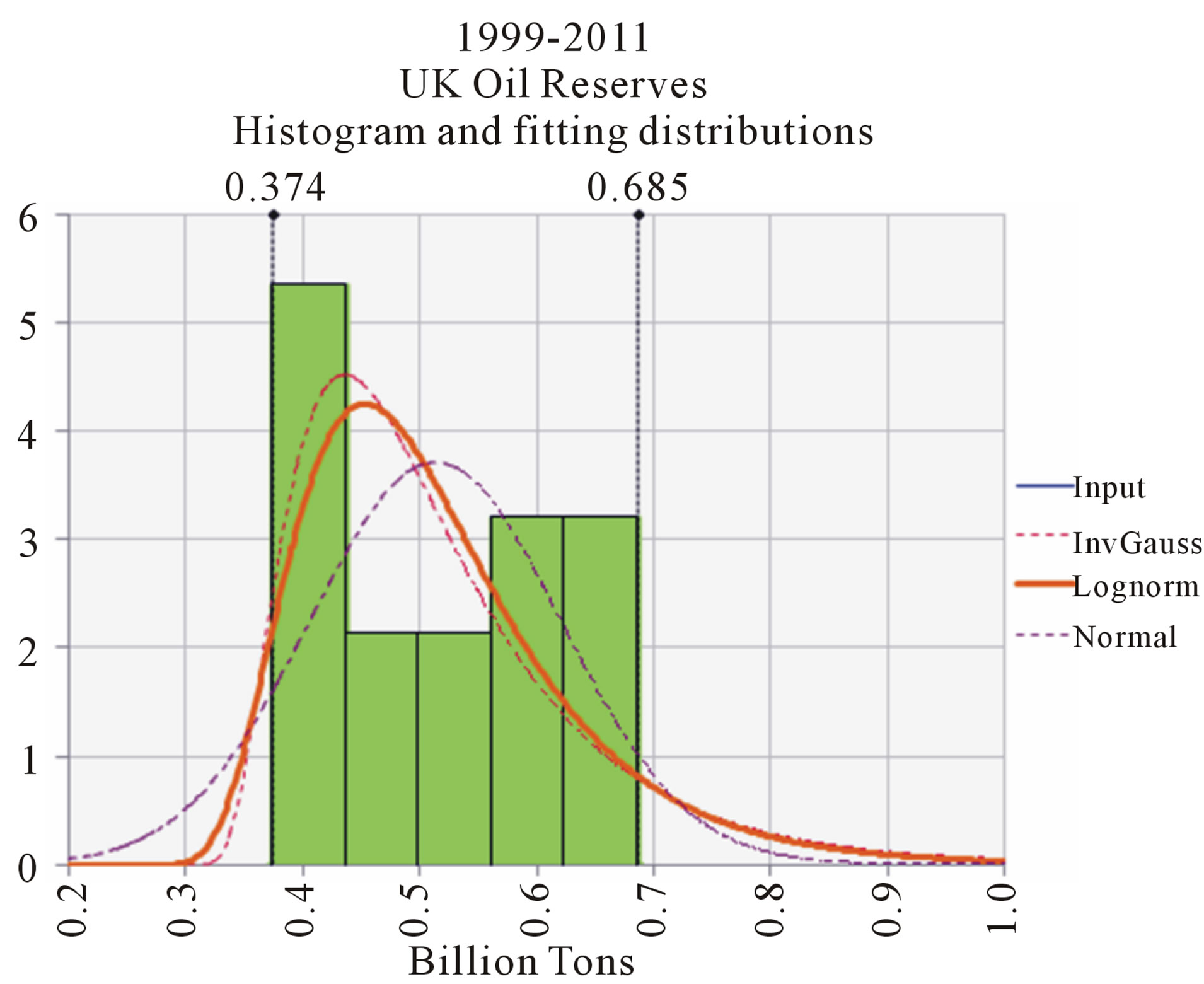
Figure 3. 1999-2012. UK Oil Reserves. Histogram and probabilistic distributions.
b) The standard deviation of the distribution is determined as the product of multiplying the mean value times the Coefficient of Variation for the respective data.
8) Run a Montecarlo simulation over the time interval until convergence is reached.
9) The results of the simulation are presented in probabilistic bidimensional charts.
10)Experimentally designed test are performed with the analysis of the likely value of the variables involved in the EMPF to imitate the output of conventional forecasts or any other scenario worth of investigation.
3.1. Case Study Based on the Official Data of UK Oil Reserves
The following data comes from the UK official source of information on Oil and Gas [3]
The reserves for 2012 are extrapolated from the data of the previous years (1999-2012) according to the best polynomial fitted equation:
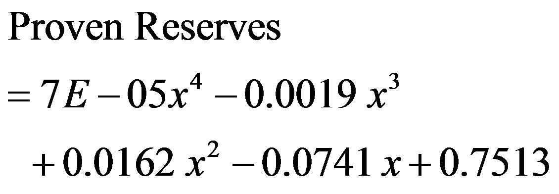 (8)
(8)
The values of variable x are integers in the range of 1 to 15, the interval of years between 1999 and 2012.
In Figure 4, it is appreciated the display of the official data of proven reserves by year, with a clear dominant declining trend up to 2010.
From the information provided by Table 1, the calculated statistic parameters we will use for the simulation are:
In Table 2 the descriptive statistic of relevant parameters calculated from the data in Table 1 are referenced.
The segmented lines in Figure 5 are according to: the official projection (red segmented line), the modified exponential fit projection (segmented light green line), and a projection based on the method and EMPF (segmented blue line)
A bidimensional forecast, or summary graph, can be produce with the aid of the software @Risk, after running the montecarlo simulation in microsoft Excel. The yellow line in Figure 6 indicates the most likely or average outcome of oil production after running the montecarlo simulation according to the settings provided to the variables of the EMPF.
The statistical record of outputs of the simulation al-
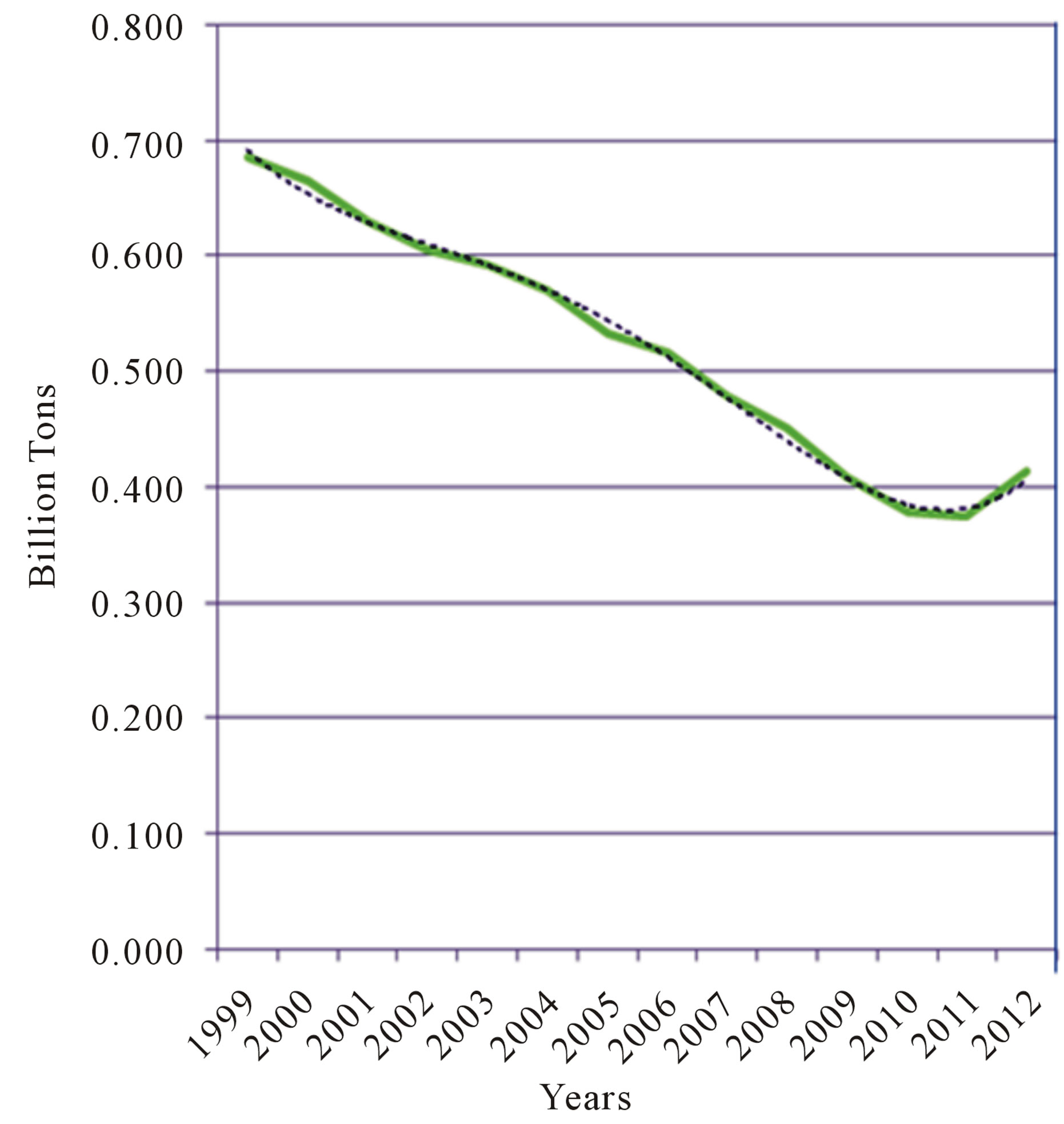
Figure 4. UK Proven Reserves. Plot of the data from 1999 to 2012, (green line) and the best fourth order polynomial fit (segmented black line).
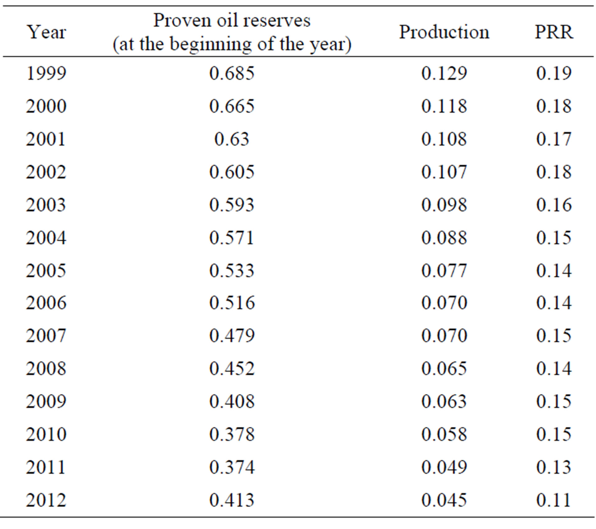
Table 1. 1999-2012 Production reserves ratios based on UK Official record of production and proven reserves [3]. Units in Billions of Tons.
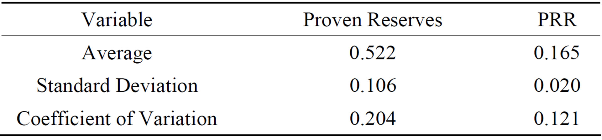
Table 2. Statistical parameters for the reserves and the PRR according to the analysis of the 1998-2011 dataset.
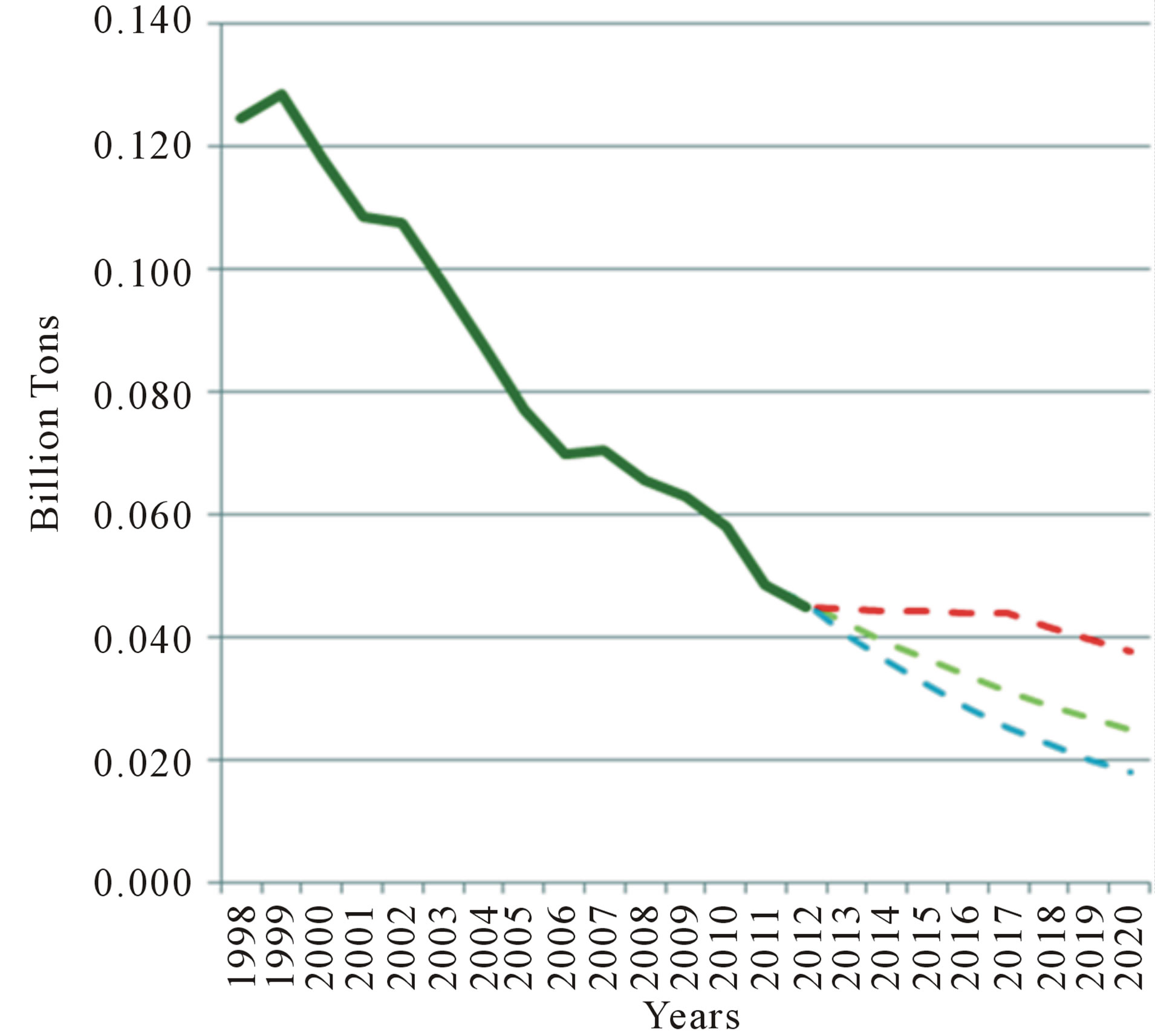
Figure 5. Line chart integrating the record of UK known oil production from 1998 up to 2012 (continuous dark green line) with different projections for 2013-2020 (segmented lines).
lows to make probabilistic intervals of confidence for the mean value of the production for every year. The inner interval provides a interval of confidence one standard deviation above and below the average value where the simulation converged. So there is around 66% of probability the size of the output of production be inside this inner band. The Outermost band provides 90% of probability for the interval of confidence.
So, taking advantage of working with two dimensional forecasts as in Figure 6 lets appreciate the range of values the production could end up under a probabilistic window. The Official and Exponential Fit forecasts (red and green segmented lines in Figure 6) are included for comparison For instance, for 2013 there is 90% probability the production of oil be between 0.058 and 0.027 Billion Tons. By 2020, the range of values for the same probability window drops between 0.025 and 0.011 Billion Tons.
The official forecast, however, only keeps inside the 90% probability window until 2015. By other hand, the forecast based on the exponential trend stays inside the 90% probability window even until 2020.
Experimental Design
The following example illustrates how the EMPF can be applied to obtain planned production commitments. As deducted from the report by [4], the official 2013-2020 production forecast for the UK points at a cumulative production of 340 Billion Tons. To achieve this goal under the settings provided by the EMPF we could proceed in several ways. We will follow either ED1) How much the average PRR should be increased to achieve 340 BT of cumulative production, considering the Proven Reserves are depleted from the levels accounted by 2012?
ED2) How much the average Proven Reserves should be increased to achieve 340 BT of Cumulative Production, considering a PRR keeping an average conservative value?
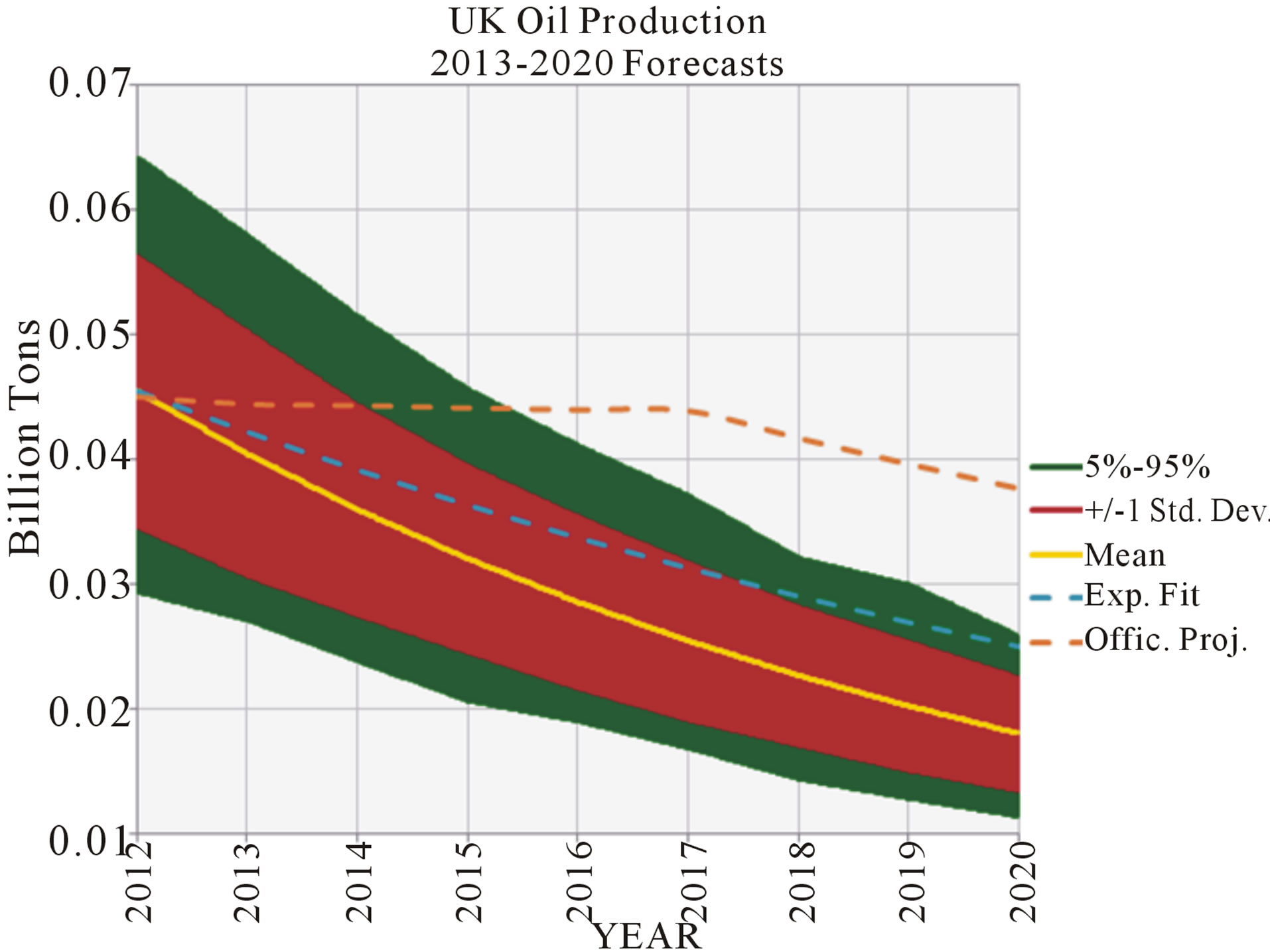
Figure 6. UK Oil Production 2012-2020. Two dimensional forecast based on the EMPF.
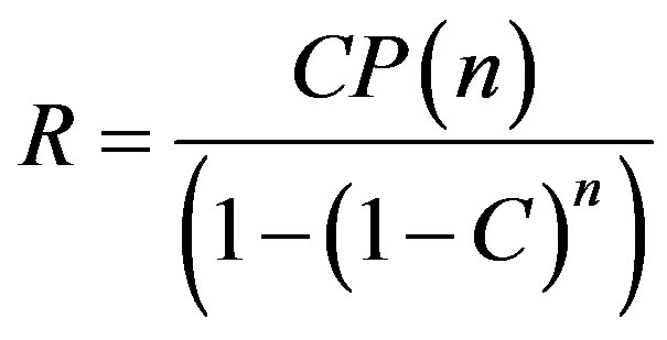
![]() To answer the questions, we use Equation (3) as follows:
To answer the questions, we use Equation (3) as follows:
R/ED1)
 (9)
(9)
In this case, we replace CP(8) by 0.340 BT, R by 0.368 BT and n by 8.
The answer is C = 0.274 R/ED2)
 (10)
(10)
In this case, we replace CP(8) by 0.340 BT, C by 0.17 BT and n by 8.
So, the available amount of reserves to develop from 2013 would be 0.439 BT, what is an increase of 0.071 BT over the current amount of proven reserves by 2012.
3.2. Case Study Based of Nevada’s Official Data of Gold Reserves and Production
The following official information at Table 3 is taken from the Special Publications of the Nevada Bureau of Mines and Geology [5].
The descriptive statistic analysis of the data, provided in Table 4 indicates the distribution of gold reserves is well centered around the average value of 75 MM t Oz.
The histogram in Figure 7 is well fitted by the exponential and lognormal distributions. Although the best fit with triangular distribution is not as good as the lognor mal or exponential, it has the advantage of a smaller Coefficient of Variation. For the years under study the reserves have 90% probability of being between 64.0 to 90.1 MM t Oz.
As a first conventional approach for the modeling, the historical data fits well a linear correlation (Figure 8):
 (11)
(11)
The values of variable x are integers in the range of 1 to 10, the interval of years between 2001 and 2010.
After applying the methodology explained in previous sections it came up the following scenario’s insights for the bidimensional forecast (see Figure 9).
First, evaluating the range of values the production could end up under a 90% probabilistic window we find that:
The segmented line, corresponding to the forecast based on the conventional lineal correlation (Equation (11)), stays inside the envelope provided by one standard deviation range of probabilities (approximately 66% probability range).
For 2013 there is 90% probability the production of gold be between 6.2 and 2.5 MM t oz.
By 2015, and for the same range of probabilities, the likely production goes down to the range between5.5 and 2.3 MM t oz.

Table 3. Nevada state. PRR calculated from the record of gold production and reserves. Figures in MM Troy Oz.
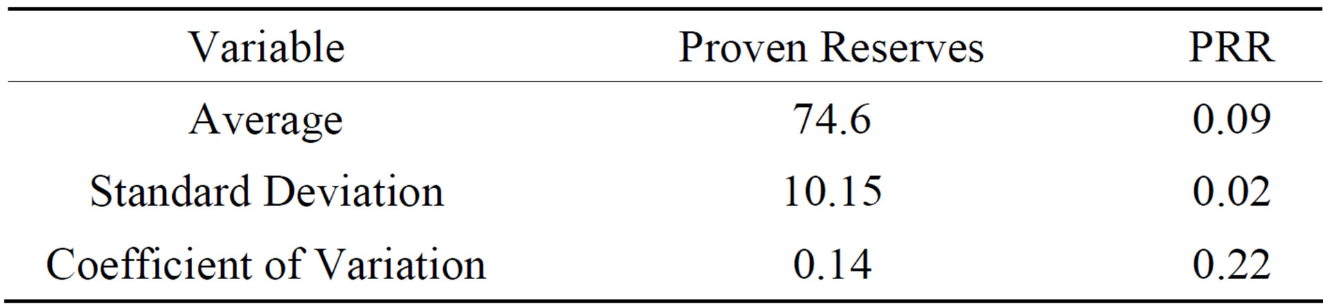
Table 4. Statistical parameters for the reserves of gold in Nevada and the PRR according to the analysis of the 2000- 2010 dataset.

Figure 7. Nevada state. Histogram and probabilistic distributions of gold reserves from 2000 to 2010.
Experimental Design
Under contemporary conditions and booked reserves, the 2011 official report indicates an estimate of 15 years of sustainable gold production at current levels.
As we see for simple inspection of the exiting proven reserves, the current level of production is sustainable until the reserves left are around 5 MM t Oz, in the order of 10% of the current booked volume.
In this case, after 15 years the ratio Cumulative Production over Reserves would be around PA/R = 0.90. We could use Equation (3) to determine the average PRR
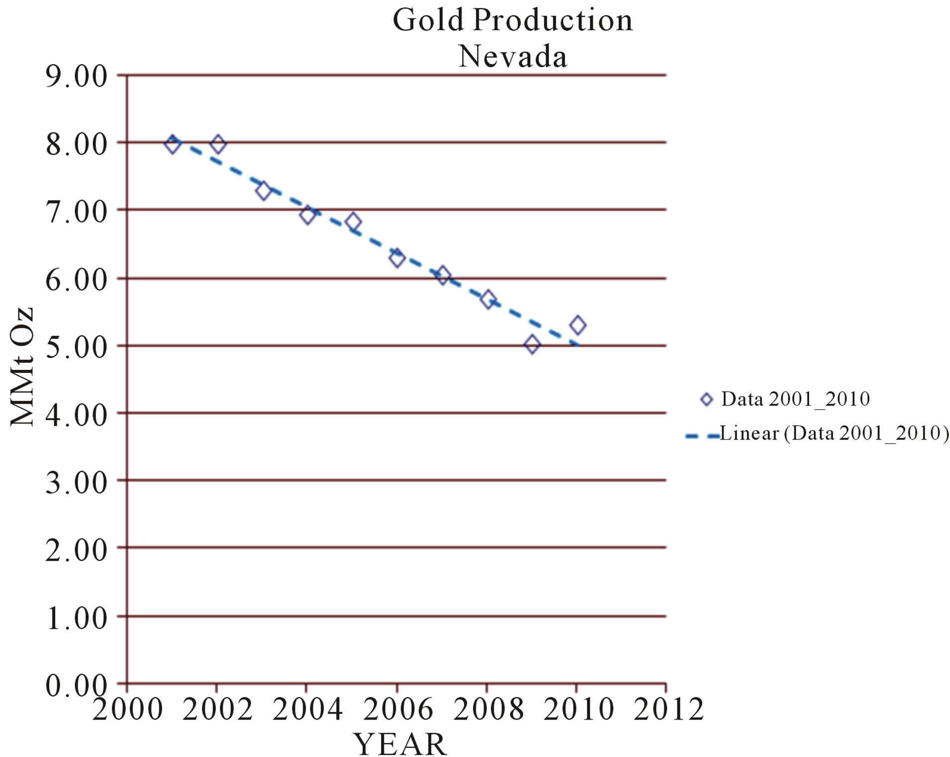
Figure 8. Plot of historical data of gold production and its lineal correlation (segmented line).
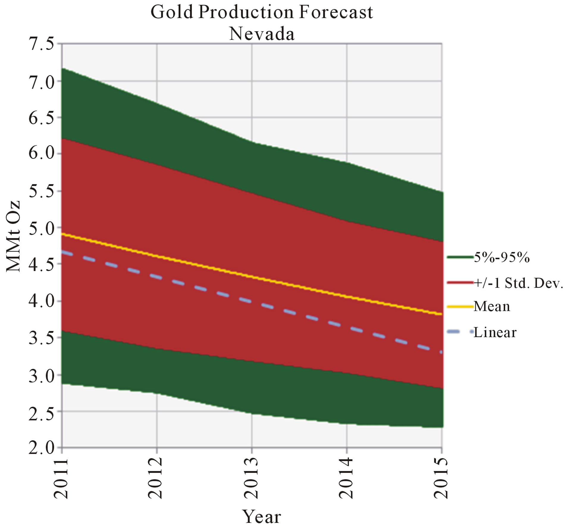
Figure 9. Nevada state. Bidimensional and lineal conventional forecast for the production of gold from 2011 to 2015.
required to accumulate 90% of the current reserves after 15 years:
 (12)
(12)
Replacing n by 15 and PA/R by 0.90, we get C = 0.14.
Although seems a conservative value, the historical trend of PPR does not support to expect for the PRR a grow of such magnitude (a factor of 1.75) in the short term.
However, this is a conservative value compared with the average PRR required to keep producing 5 MM t Oz for more than ten years (0.3 from Table 5).
It seems more reasonable for the PRR to grow steadily with time for the current level of production to be sus-
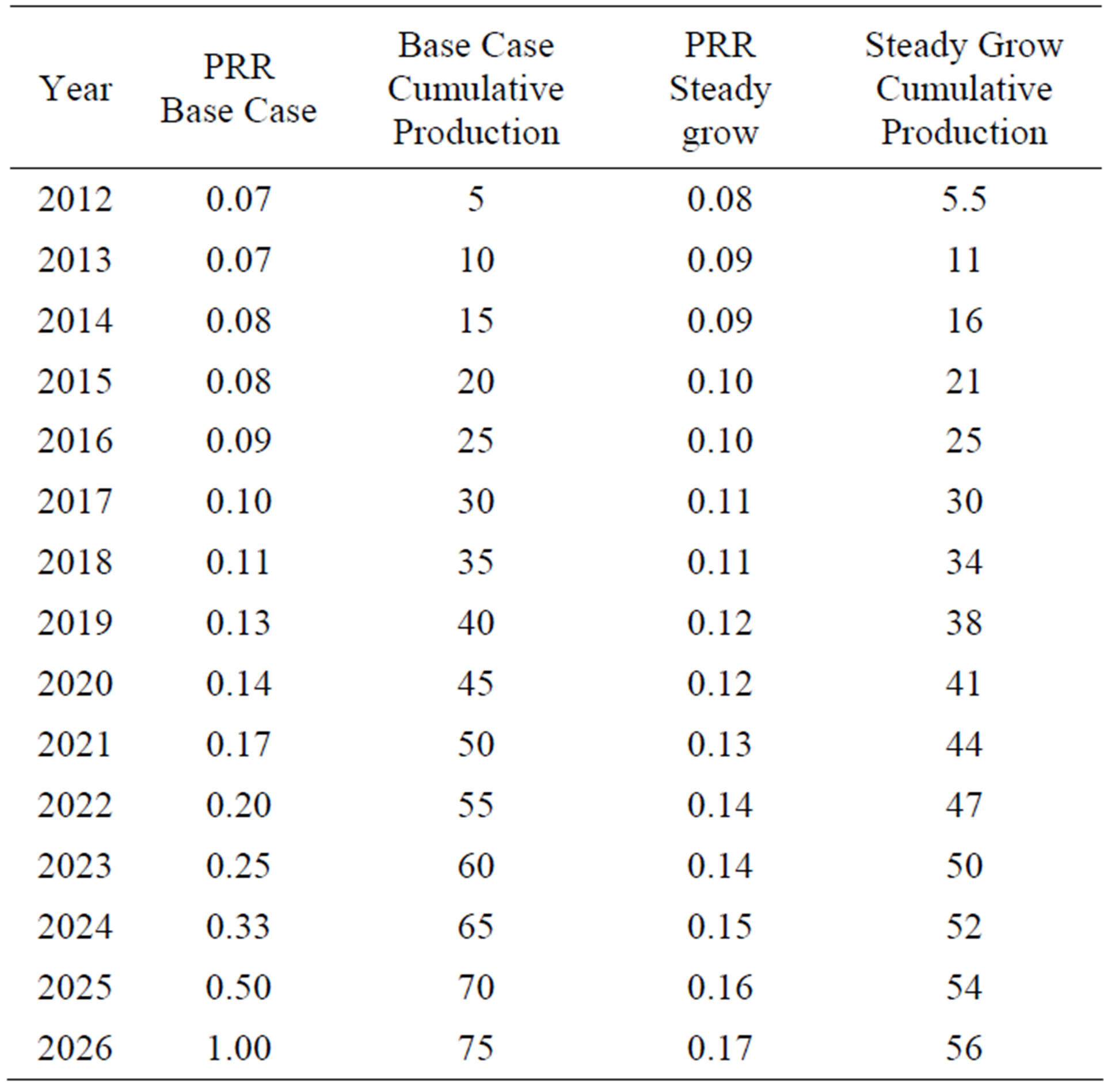
Table 5. Projections of gold outputs 2012 to 2026. Comparison of the PRR and the cumulative production of gold following a either a fixed quota of 5 MM t Oz or a variable quota controlled by a PRR with a steady grow.
tained.
Under these premises, the PRR in Equations (2) and (3) can be modified to account for a constant increase by a factor of over n years under simulation. Notice that for Equations (14) and (15), n must be greater than one:
 (13)
(13)
![]() If n = 1:
If n = 1:
If n > 1:
 (14)
(14)
If n= 1:
If n > 1:
 (15)
(15)
In Table 5, the Base Case of 75 MM t Oz of reserves depleted under a sustained production rate of 5 MM t Oz is compared with the output of a conservative depletion under a 5% grow of the PRR from one year to the next. To model the steady grow of the PRR it is used Equation (14).
It can be noticed that after 15 years the production under a steady grow manages to accumulate 75% of the initial reserves. The PRR experiences a moderate twofold grow. The base case, by other hand, follows an aggressive tenfold grow to exhaust in 2026 the reserves available by 2012. It implies a increase of one order of magnitude in a decade and a half.
These results open an experimental way to explore a reasonable competence between the depletion of reserves and the grow of the PRR to keep a given rate of production.
4. Discussion
With the results provided by the cases under study we notice how the methodology and equations presented have a widespread range of applications to forecast mineral production at any scale. The universal and multi scale capabilities of the equations rely on the fundamental principle of the conservation of matter, what is produced equals what is extracted from the reservoirs.
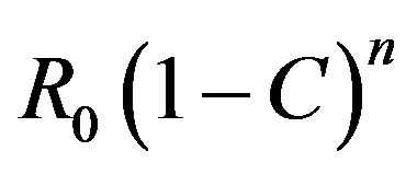
One point to argue about the cases under study is that the equations are applied to model late stages of production. The definition of Equation (1), with a constant (CR0), multiplied by a factor smaller than one (1-C) raised to the years since the start of production, suits well a trend of declining resources. The modeling of the early step up and the plateau of production require further developments of the EMPF and are left for later study.
To model production outputs based on the EMPF requires some care with the validation of the data that supplies the statistical entries of the variables. Although official data from private or public entities are disclosed under the assumption of a internal quality control, it is suggested as a rule of safety to apply to the data the criteria to evaluate the information [6]. It will, in general, increase the confidence on the results, what is especially important considering that figures of mineral reserves are quite sensitive to be over or underestimated. Regarding the study cases the input data of the EMPF, provided by official entities, is assumed as objective and reliable. However, when the reliability of the data is under scrutiny, additional work over the information might be done, via the indexes of reliability, like the Alpha of Cronbach or the coefficients KR-20 and 21 of Kuder and Richardson [7]
The record of more than a decade of information is enough to apply the chi square test to fit distributions to the data, for what the condition of sufficiency to model the distributions is fulfilled. With less than five measurements this is not possible.
Depending upon the statistical parameters calculated from the data, every case would have the need of information of different sizes of samples of years of production and the correspondent record of proven reserves, to apply the methodology and equations presented with a certain degree of certainty.
The treatment of the variables during experimental design makes possible to account for conditions not included in the historical record of production and estimation of reserves. These experimental or trial conditions could alter the historic pattern driven by the statistical record. The mathematical link between the variables involved in the EMPF gives adequate room to do so. At this point it stands out the intrinsic value provided by the EMPF. The connection between time and changes of the variables reserves and production gives the EMPF a versatility that makes them especially suitable for forecasting purposes.
Strategic plans answer to questions as how much of the domestic demand it will be meet by the domestic supply and hence how much should be imported, with all the implications over the budget of the entity.
It has been usual to support production commitments based on scheduled operational actions. These could be increasing the input of fluids from new drillings at areas with proven undeveloped reserves, or executing plans for workovers and well repairements of handicapped wells with a delayed production potential, among others. Although these expectations could be met if plans to keep up or increase production are well executed, the statistical behavior of the production with time should also be accounted as a control variable to visualize outcomes of future production.
How to deal in a practical way with the application of PRR to forecast field, corporative, country or even regional production? As experience shows, at these scales Reserves, Production rates and (consequently), PRR change with time. For instance, production rates could be modified to allow aggressive business plans to take over markets flooded with soaring oil prices. Reserves are recalculated every year as a function of new discoveries, adjusts and enhancements from new models of oil reservoirs. This could lead not only to engrossed figures, but also to significant drops in corporative assets when bogus reserves are discarded.
The statistically oriented method set aside to give a pragmatic use of the EMPF is open and flexible. New improved methodologies can be developed for dedicated researchers to enhance the accomplishment of the results.
The advantage of using the method and EMPF is that not only allows to account the results of the trend imposed by the current statistical behavior of the production with time, but also, with appropriate experimental design adjustments, to account the results of actions modifying the likely results imposed by statistical trends.
As for many corporations or oil companies, national or not, the official projections of oil production represents a commitment that, for instance, can be strongly based on tactical operational actions led by the highest level of management. However, the real trend of production follows a path that can be modified under especially effective tactical operative conditions, like the incorporation of significant amounts of undeveloped proven reserves to the production output.
Otherwise, the production will tend to follow the statistical pattern already established. The method and EMPF, and even a regular functional fit of the available data, shows for overconfident business plans the warning imposed by the burden of the behavior of real production trends.
To entities in charge of managing reserves at different scales, the equations of MPF provides the tools to be aware of unsupported production commitments and the strategic plans attached to them. Also point out what kind of conditions should come out to give to the production commitment reasonable grounds to be accomplished.
An area to consider for subsequent development is to find out a criterion, both technical and financial, for the rational and optimal development of reserves. The inverse of PRR, the reserves to production ratio (R/P), has been used in connection with development optimization and present value maximization [8]. These analyses have led to the notion of best R/P as the figures which produce the highest present value. This addresses aspects of the financial side of the analysis of the connection between reserves and its production, a subject worth of further treatment in future studies.
5. Conclusions
The study cases, one taken from the oil industry at the scale of a country, and the other for the mining industry at the scale of a national state, address the issue of exemplifying how the EMPF has a universal range of applications to model production forecasts of mineral reserves at any scale.
The modeling of cases of mature stages of mineral production shows how the EMPF work for trends with a clear declining behavior. The analysis of the applicability of the EMPF to model an early rise, a plateau or even irregular trends of production is a subject worthy of further development but it is not included in the objectives of the actual study.
The methodology and equations of mineral production forecast provide a frame of reference to diagnose the feasibility of conventional ones. They can offer a statistical frame of reference and give dimensions to the variables that shape the output of production with time.
This allows for useful tools to evaluate the statistical and practical feasibility of the forecasts based on conventional methods. Essentially, it consists on comparing how viable is the likely size of the variables provided by experimental design with the statistical records of the variables.
REFERENCES
- K. Deffeyes, “Beyond Oil. The VIew from Hubbert’s Peak,” Hill and Wang, New York, 2006.
- S. Pérez Rodríguez, R. Soto and B. D. Soto, “The Development of a New Methodology to Reduce Uncertainty in Implementing a New EOR Project,” IPTC-17017-MS, 2013
- Office for National Statistics of the United Kingdom, 2013. http://www.ons.gov.uk/ons/rel/environmental/environmental-accounts/2011/sum-oil-gas-reserves.html
- M. Earp, “UKCS Oil and Gas Production Projections,” Department of Energy and Climate Change (DECC), 2013.
- Nevada Commission on Mineral Resources, 2011. http://minerals.state.nv.us/forms/mining/MajorMinesOfNevada/
- M. Namakforoosh, “Metodología de la Investigación,” 2nd Edition, Limusa, Mexico, 2011.
- R. Hernández, C. Fernández and P. Baptista, “Metodología de la Investigación,” 5th Edition, McGraw Hill, 2010.
- I. Hayhow and G. J. Lemee, “Reserves to Production Ratios and Present Value Relationships,” 2000 SPE/CERI Gas Technology Symposium, Calgary, 3-5 April 2000. doi:10.2118/59783-MS
- I. Sominsky, “Method of Mathematical Induction,” D C Heath & Co., 2000.
ANNEX. 1
Proof by induction the Reserves (R(n)) for year n are equal to
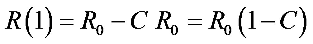
Theorem 1: For n = 1 the hypothesis is valid since
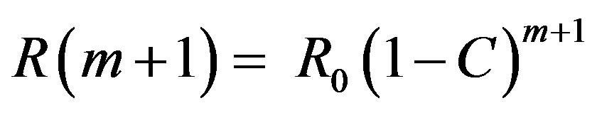
Theorem 2: Let’s suppose the hypothesis is valid for n = m, what means:

where m is a natural number.
Lets show the hypothesis is valid for n = m + 1, that is
That it is true since
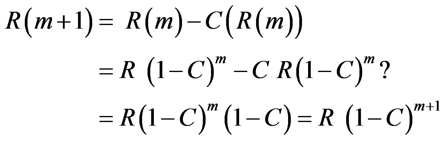
Having demonstrated Theorems 1 and 2 we can rely on the principle of mathematical induction [9] to sustain