American Journal of Computational Mathematics
Vol.3 No.4(2013), Article ID:39768,6 pages DOI:10.4236/ajcm.2013.34038
A New Recombination Tree Algorithm for Mean-Reverting Interest-Rate Dynamics
Department of Mathematical Sciences & Financial Engineering Program, Stevens Institute of Technology, Hoboken, USA
Email: peter.lin@stevens.edu
Copyright © 2013 Peter C. L. Lin. This is an open access article distributed under the Creative Commons Attribution License, which permits unrestricted use, distribution, and reproduction in any medium, provided the original work is properly cited.
Received June 13, 2013; revised August 15, 2013; accepted September 12, 2013
Keywords: Natural Asset; Financial Value; Neural Network
ABSTRACT
In light of the fact that no existing tree algorithms can guarantee the recombination property for general OrnsteinUhlenbeck processes with time-dependent parameters, a new trinomial recombination-tree algorithm is designed in this research. The proposed algorithm enhances the existing mechanisms in interest-rate modelings with the comparisons to [1,2] methodologies, and the proposed framework provides a more efficient way in discrete-time mean-reverting simulations.
1. Introduction
A general Ornstein-Uhlenbeck process is defined such that
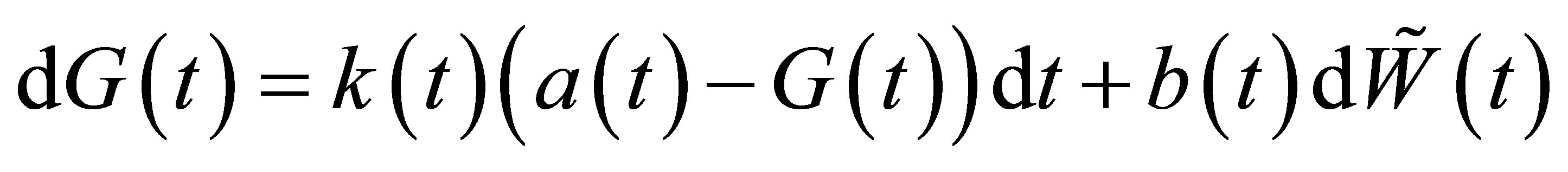
where  is a standard Brownian motion, and
 ,
,  ,
,  are time-dependent deterministic parameters. The parameter
  is the mean-reversion term indicating the long-term mean-reverting level with a rate
  at time t. The source of randomness is described by the Brownian motion
  multiplied by a volatility term
 .
.
A tree is an acyclic structure where each node has zero to multiple descendant nodes and one parent node. A recombination tree is a special tree structure of which the size grows linearly. Therefore the investing decisions, if computed recursively, have time complexity1 at most , which is much more efficient than a general simulation method which may cost exponential amount of time. For example, a recombination tree can help us to efficiently determine the price and the buy/sell timing for an American style option by comparing the derivatives value at each tree node with its children nodes (see [4] for more details). However, designing a recombination tree algorithm for modeling interest rates is far from trivial. Here are two examples:
In [1], Hull and White provided a heuristic two-stage method for constructing an interest rate tree based on the extended-Vasicek short-rate model.2 In the first stage the algorithm builds the framework of the tree, and in the second stage the algorithm calibrates the tree to the current interest-rate term structure. The algorithm is designed for a short-rate model; hence the tree cannot be adjusted or updated according to the markets. Also, their method cannot deal with stochastic mean-reverting parameters, and there is no guarantee that the tree is a recombination tree especially when the volatility term of the short-rate process is a decreasing function. Therefore, Hull-White’s algorithm is not a good candidate.
In [2], Black, Derman, and Toy (BDT hereafter) also provided a recombination tree algorithm for short rates. Their tree is constructed recursively and calibrated to zero-coupon bond volatilities and current interest rate structure. Though the BDT tree guarantees a recombination structure, the tree is not designed for a general Ornstein-Uhlenbeck process. Therefore, the BDT tree is not a good candidate either.
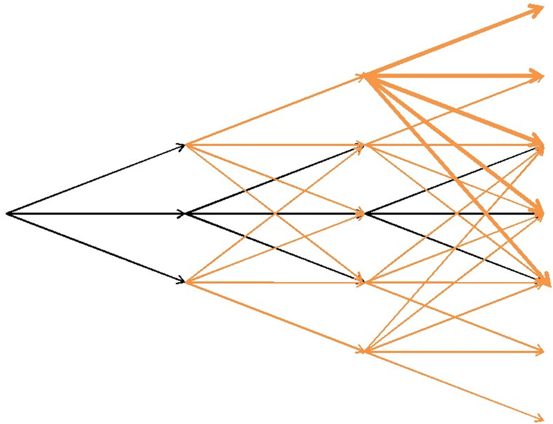
In light of the fact that no existing tree algorithms can guarantee the recombination property for general Ornstein-Uhlenbeck processes, we propose a new recombination trinominal tree algorithm. The idea is to modify a standard trinominal tree(Exhibit 1(a)) by adding extra branches at each node. First, we denote the tree structure in black color the center path. Then, given a node  directly above (below) the center path, define
  the set of nodes containing
  and all the nodes down to (up to) the center path. Then we modify the tree according to the following rules: 1) the center path remains unchanged; 2) given a node
  above the center path, we connect the node to all the descendant (children) nodes stemming from
 ; 3) given a node
  below the center path, we connect the node to all the descendant nodes stemming from all the nodes from
 . The modified tree structure is shown in Exhibit 1(b). We will use the names, spanning nodes and spanning branches, to identify those nodes not on the center path, and branches not emanating from a center node.
The crucial key of modifying a standard trinominal tree is that we can further simplify and still keep the tree structure by adding sibling branches. Sibling branches are one-way streets through which we can only move up or down at a given time epoch, but not in both directions. A spanning node above the center path can reach the center path and all the nodes in between only by moving down through the sibling branches; a spanning node below the center path can reach the center path and all the nodes in between only by moving up through the sibling branches. As a result, by adding the sibling branches, each node can reach all but one descendent nodes via its sibling branches. So, in the simplified tree structure, each spanning node will have only one time transition descendant branch. The final tree structure is shown in Exhibit 1(c) . The algorithm is given below. The proof of the correctness of the algorithm for simulation is given in Section 3.
2. Algorithm
Now we give a full description of the algorithm. Let  denote the node on the center path at time
 , and let
  denote the value of node
 . Therefore, if
  is represented as a function, then it indicates the value of the node. Let
  and
and  denote the k-th node above center node
  and the value of
  respectively. Similarly, let
  and
and  denote the k-th node below center node
  and the value of
  respectively. Moreover, if we use capital letter
 , then it represents a random variable of the tree value at time
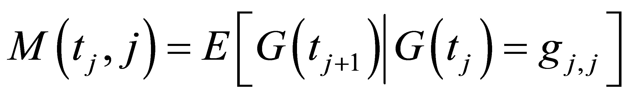
 . To shorthand the notation, the expectation value
  conditional on the position of
  is written as
 (1)
(1)
Define the conditional expectation at node  to be
to be
 (2)
(2)
Since the volatility term in stochastic-splines model is assumed to be a deterministic function, the conditional variance is the same for all nodes at a given time, i.e. at time , the conditional variance
 (a)
(a)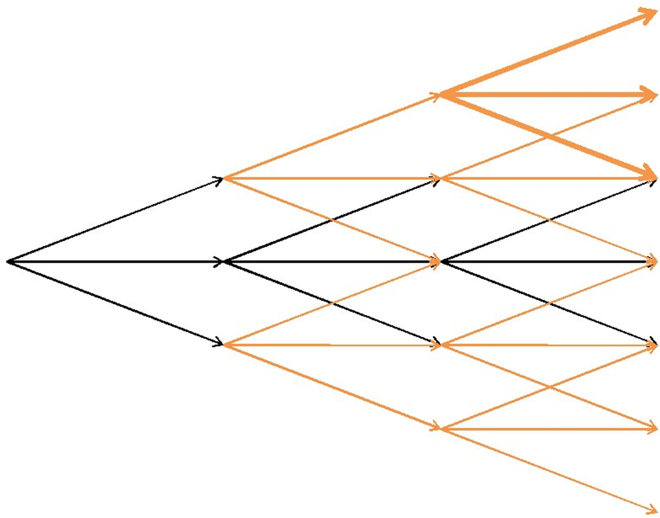 (b)
(b)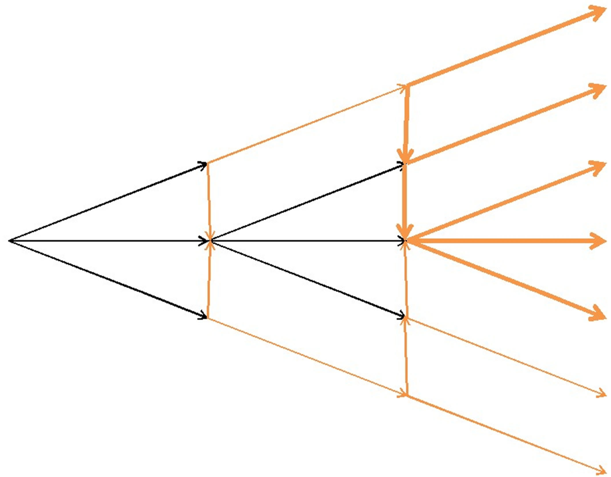 (c)
(c)
Exhibit 1 . (a) original recombination trinominal tree; (b) modified tree; (c) simplified Tree.
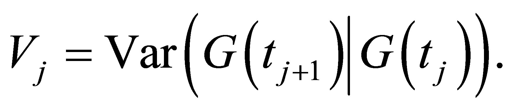 (3)
(3)
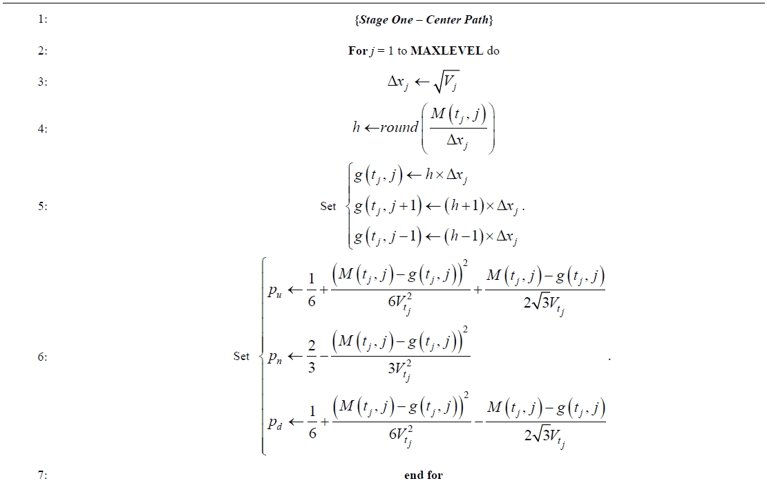
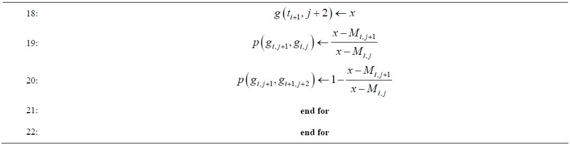
The idea of the recombination algorithm is to construct the center path first including the node values and branch probabilities, then determine the values of the spanning nodes, the probabilities on the spanning branches, and the probabilities on the sibling branches. The details are given in Algorithm 1. However, the algorithmshows that each tree is designed for simulating one coefficient process; if we have N coefficient, we will need to build N trees altogether if coefficient processes are correlated. After constructing the coefficient recombination “forest”, we can simulate the interest rate curve efficiently.
The justification of the algorithm is given in the next Section.
3. Verification
First we look at the first part of the algorithm and some notations. The first stage of the algorithm follows the standard Hull-White methodology (see [1]) and provides the backbone of the tree. Let  denote the node on the center path at time
 , and let
  denote the value of node
 . Therefore, if
  is represented as a function, then it indicate the value of the node. Let
  and
and  denote the k-th node above center node
  and the value of
  respectively. Similarly, let
  and
and  denote the k-th node below center node
  and the value of
  respectively. Moreover, if we use capital letter
 , then it represents a random variable of the tree value at time
 . To shorthand the notation, the expected value
  conditional on the position of
  is written as
 (4)
(4)
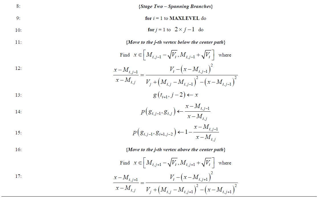
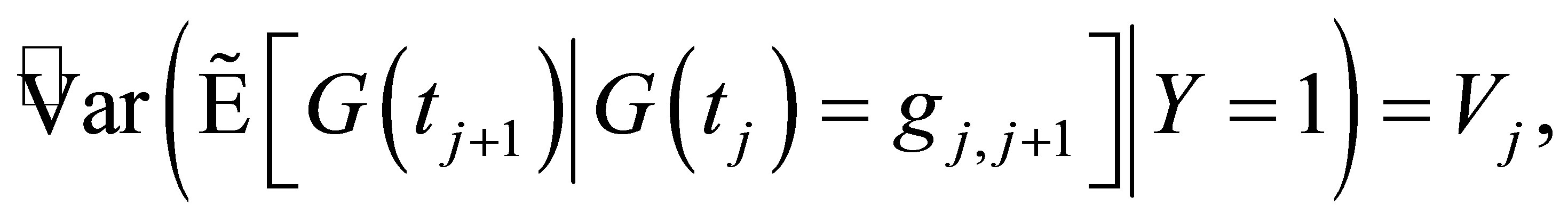
Now we move to the second part of the algorithm. The tree branches besides the central path are called spanning branches and spanning nodes. The second stage of the algorithm adopts the ideas of the law of total expectations and the law of total variances to assign the values and probabilities of spanning nodes and branches. The procedure is done recursively. Therefore we just need to look at the cases when  and
and . Given a node
  spanning from node
  at time
 , we denote the conditional expectation and conditional variance at node
  to be
to be  and
and  respectively. Denote the probability
  to be the probability moving down from
  to
to  and
and  to be the probability moving through the spanning branch from
  to
to .
.
We can recall the law of total expectation which states
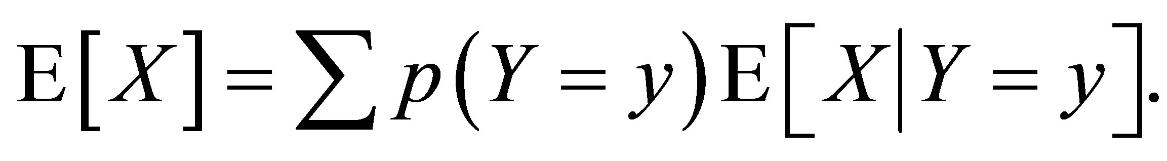 (5)
(5)
If we let
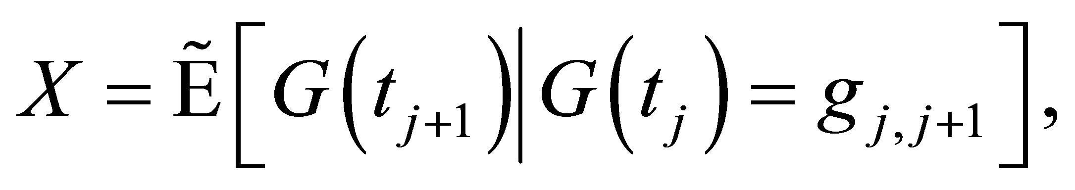 (6)
(6)
and Y denotes the random variable such that
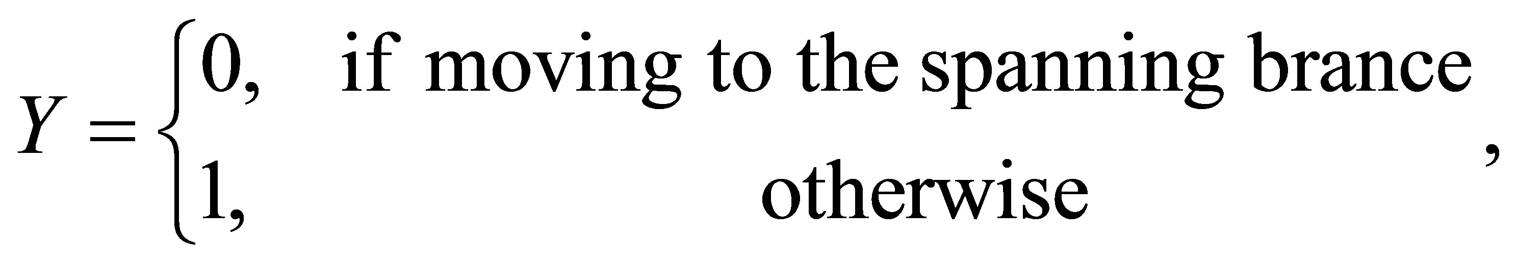 (7)
(7)
then
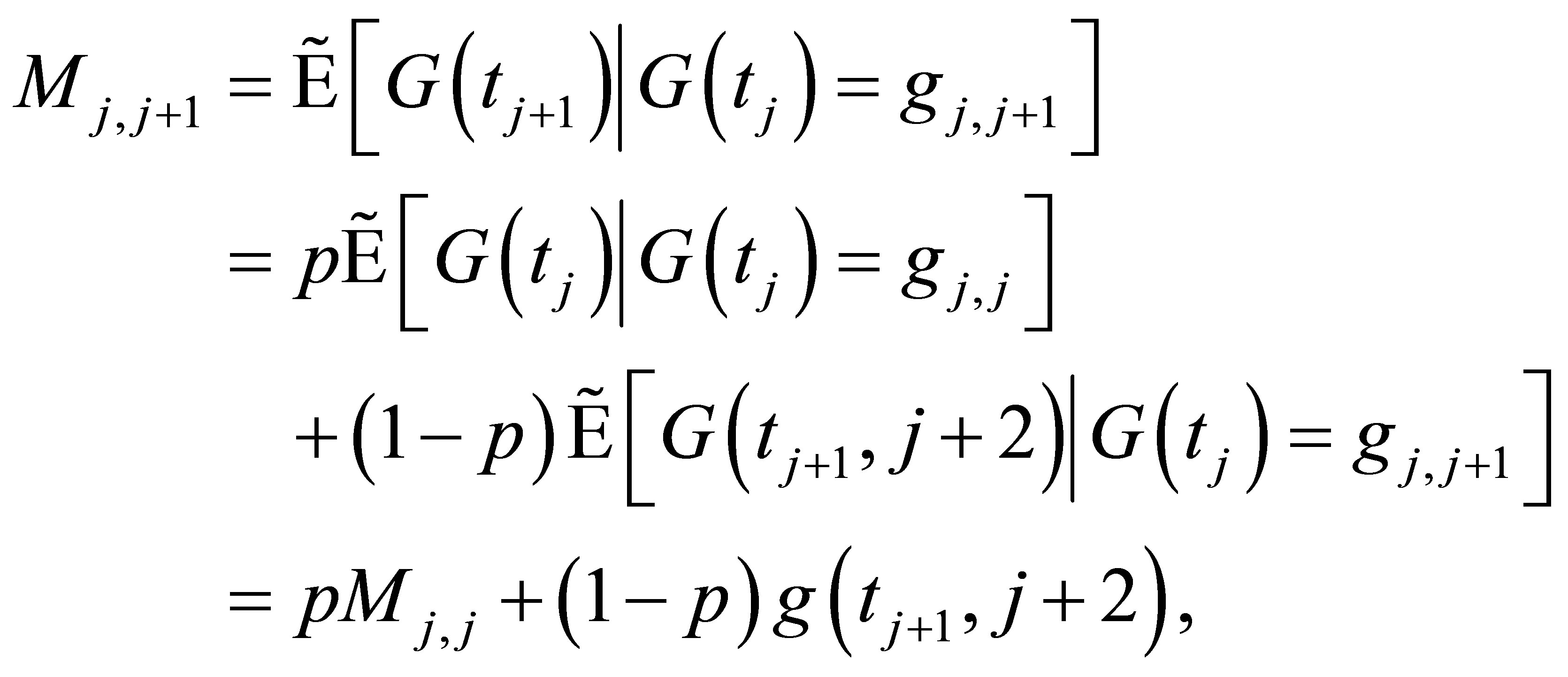 (8)
(8)
which shows
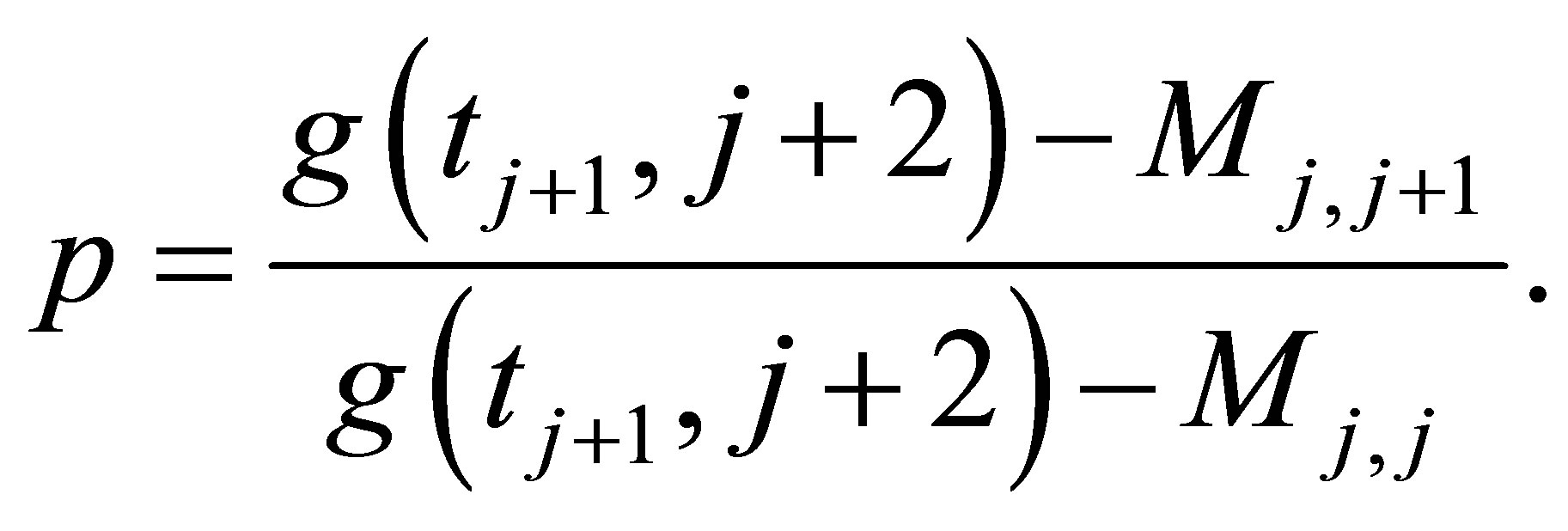 (9)
(9)
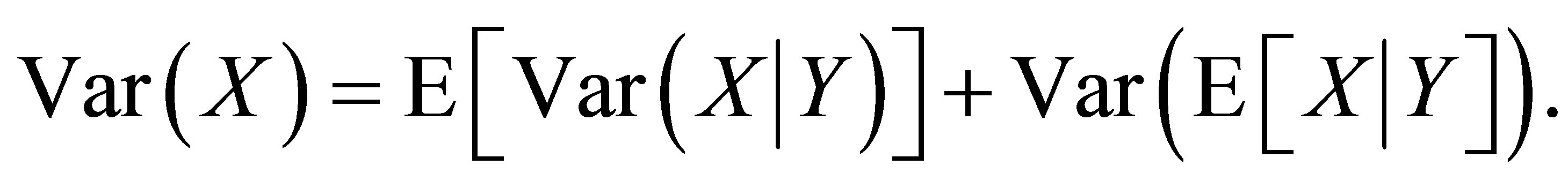
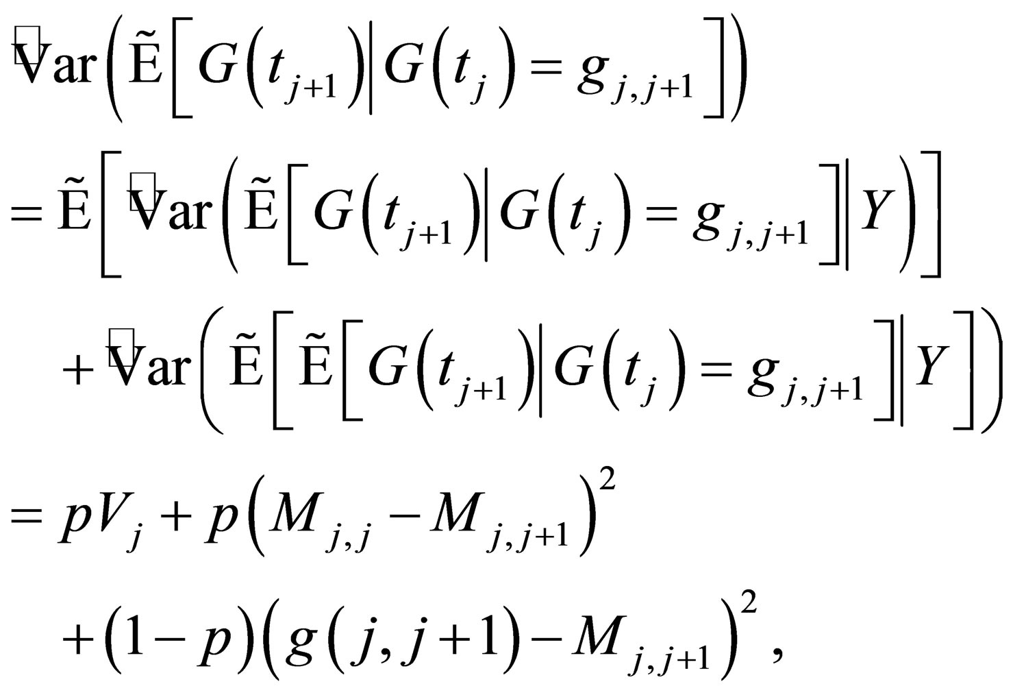
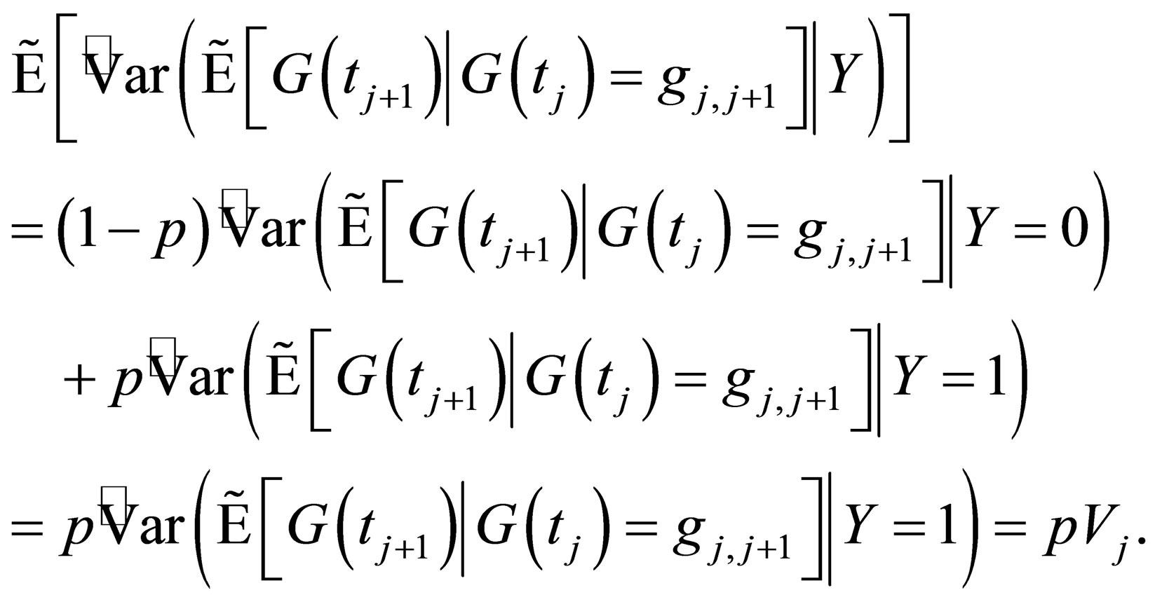
The task of deriving the relationship between  and p from the law of total variance is more complicated. We will show the the result first, then break into each part. Recall the law of total variance which states
 (10)
(10)
Similarly we let
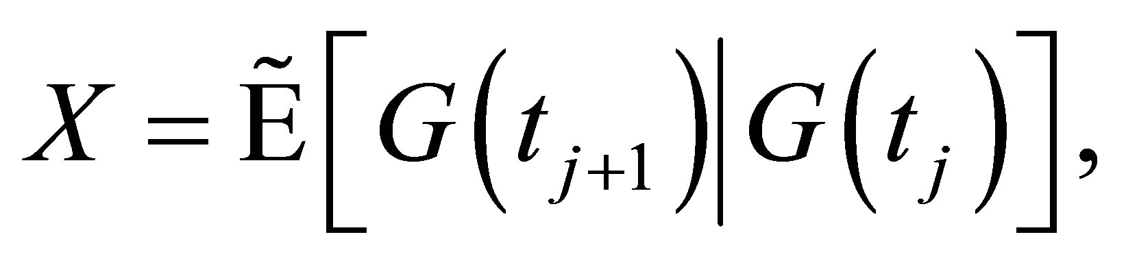 (11)
(11)
and Y denotes the random variable such that
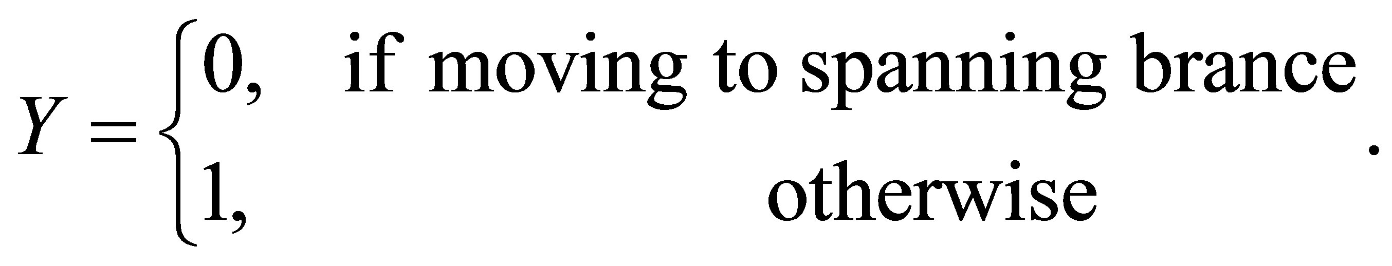 (12)
(12)
If the following statement is true:
 (13)
(13)
then we have
 (14)
(14)
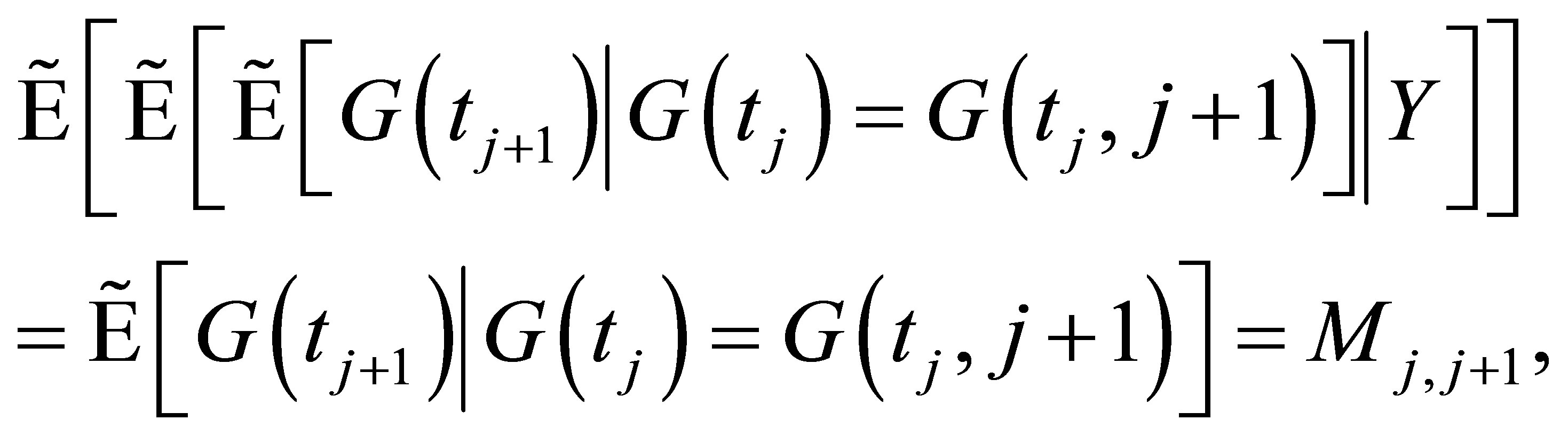
Examining the first term,  , on the right-hand-side of Equation (13),
 (15)
(15)
since there is only one choice moving from  to
to . On the other hand,
 (16)
(16)
and we know this value recursively. So
 (17)
(17)
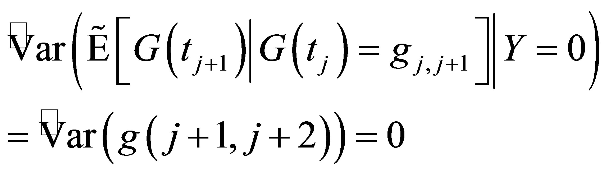
Next, the second and third terms. Since
 (18)
(18)
we have
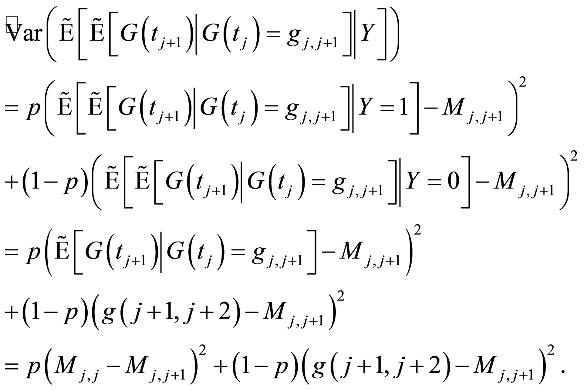 (19)
(19)
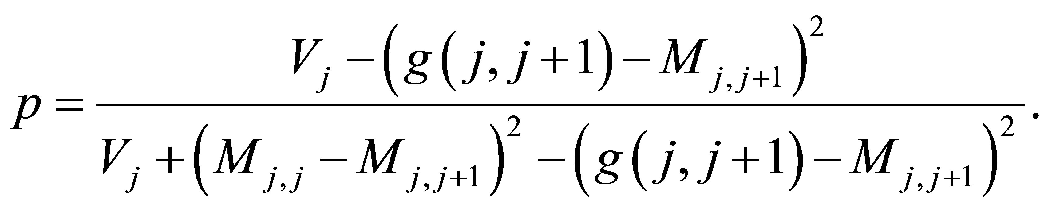
Now we have two equations and two unknown  and
and  in the following
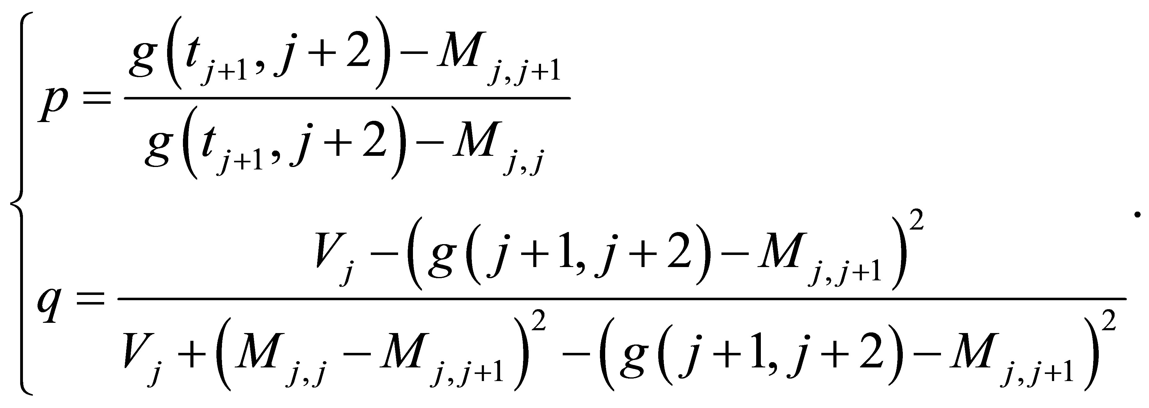 (20)
(20)
However,  must be a number between 0 and 1. And we now show that the equations indeed yield a solution such that
 . First, the case where
  and write
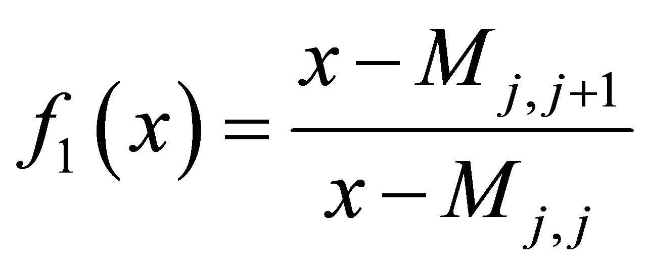 (21)
(21)
and
 (22)
(22)
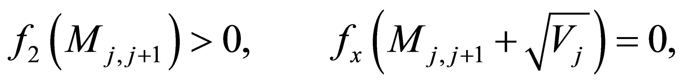
Since , for any
 (23)
(23)
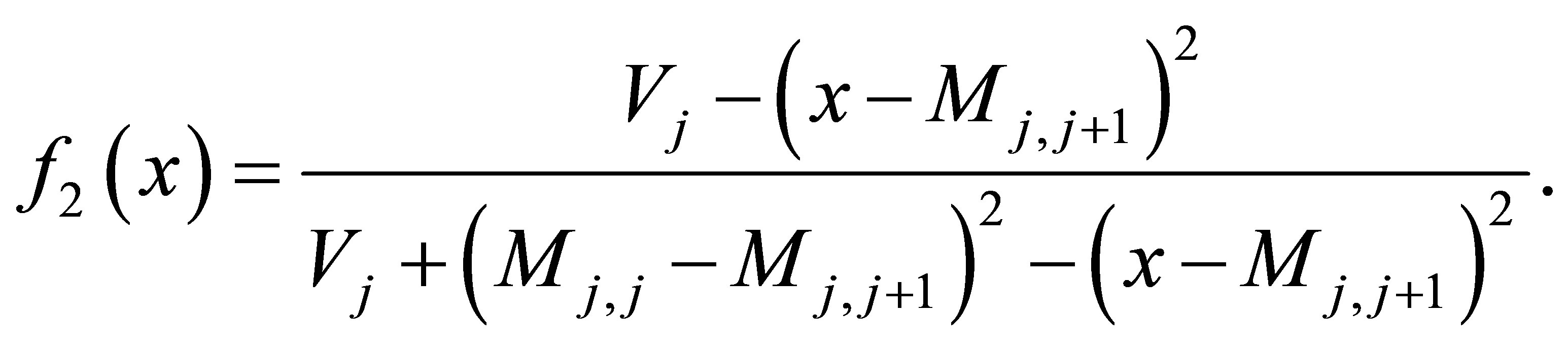
and  is continuous and monotonically increasing. On the other hand, for any
 ,
,
 (24)
(24)
and  is a continuous and monotonically decreasing function. Since
 (25)
(25)
and
 (26)
(26)
we know that there must exist a unique
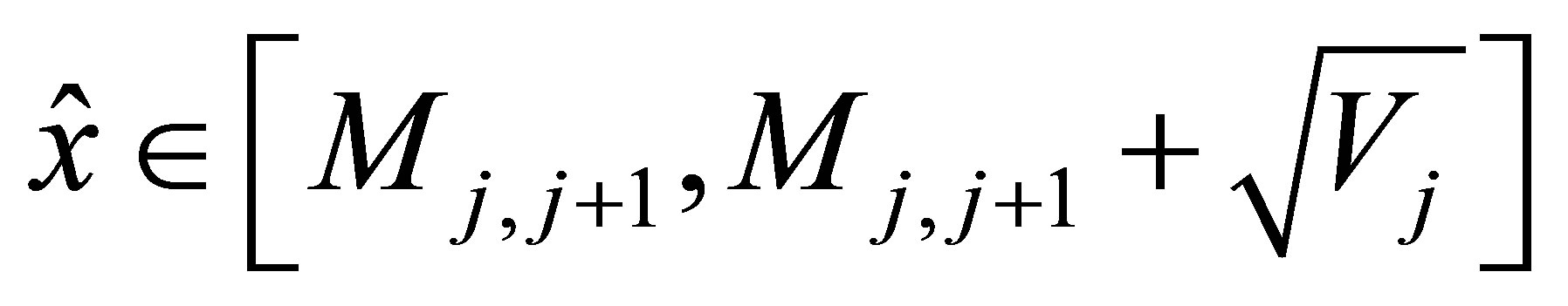 such that
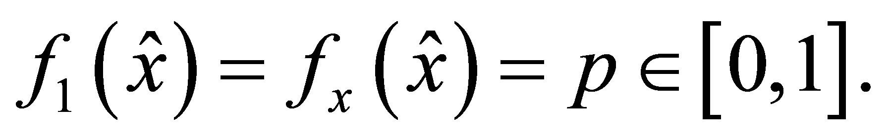 (27)
(27)
Alternatively, the proof is similar for the case when 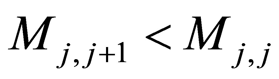 except the solution exists in
 . The uniqueness and existence of the solution
  and
and  help us solve the equations fast.
4. Conclusion
This research proposes a new trinomial recombinationtree algorithm for simulating general Ornstein-Uhlenbeck processes with time-dependent parameters. We show that there is an equivalent recombination-tree structure to simulate the mean-reverting interest-rate dynamics. Detailed algorithm and justification are given.
REFERENCES
- J. Hull and A. White, “Pricing Interest-Rate-Derivative Securities,” Review of Financial Studies, Vol. 3, No. 4, 1990, pp. 573-592. http://dx.doi.org/10.1093/rfs/3.4.573
- F. Black, E. Derman and W. Toy, “A One-Factor Model of Interest Rates and Its Application to Treasury Bond Options,” Financial Analysts Journal, Vol. 46, No. 1, 1990, pp. 33-39. http://dx.doi.org/10.2469/faj.v46.n1.33
- T. H. Cormen, C. E. Leiserson, R. L. Rivest and C. Stein, “Introduction to Algorithms,” 3rd Edition, The MIT Press, Cambridge, 2009.
- J. Hull, “Options, Futures, and Other Derivatives,” 7th Edition, Prentice Hall, Upper Saddle River, 2008.
- D. Brigo and F. Mercurio, “Interest Rate Models-Theory and Practice,” 2nd Edition, Springer, New York, 2006.
NOTES
1For the terminology of computational complexity please see [3].
2For more definitions of short-rate models, see [5]. Yet, for this article we should focus only on the mathematical modeling for general Ornstein-Uhlenbeck Processes.