American Journal of Computational Mathematics
Vol.2 No.3(2012), Article ID:23170,5 pages DOI:10.4236/ajcm.2012.23024
Numerical Modeling of the Measure of Global Environmental Needs with Applications Laser-LIDAR
1Department of physics, Université Mohamed Khider de Biskra, Biskra, Algeria
2Photonics Systems Laboratory, Université de Strasbourg, Strasbourg, France
Email: farwane@yahoo.fr
Received March 28, 2012; revised June 12, 2012; accepted June 20, 2012
Keywords: Transmission; Lasers; Optical Propagation; Atmospheric Effects
ABSTRACT
The functions of Bessel are used extensively in the various problems of the science and the technology. A laser offers practical remote sensing technologies for measuring environmental changes on both global and local scales. We describe a computer model that was developed to simulate the performance of three-dimensional (3D) laser radars (lidars). The principle of the problem consists in interpreting information on the absorption of the laser impulse in a spectral line assigned to the chemical body that one studied. Our purpose is to estimate the vertical variation of extinction and atmospheric transmission due to aerosol particles near the air-geographical surface interface. The feasibility and effectiveness of the proposed method is demonstrated by computer simulation.
1. Introduction
The measure air pollution over large European cities with lidar, mobile differential absorption lidar (DIAL). Regardless of the measures aiming to reduce the broadcasts of atmospheric pollutants, it appears indispensable all at once to improve information and to pursue the efforts of research. Systems have been developed to produce 2D and 3D maps of concentrations of nitrous oxide, nitrogen dioxide, sulfuric dioxide, and ozone. The city, concentration gradients are high and rapidly changing periods of active traffic flow (Figure 1). In absorption of light in the spectral lines of the specter often provides precious information on the properties physics of matter [1-3]. This is how the displacements of the lines (effect Doppler) inform on the speed of the movement directed of matter, and the width of the line, on the temperature and the density of this one. One uses the laser radiance extensively to determine the content of the atmosphere in different chemical bodies and sprays, and more especially to detect concentrations petty of the sparkling impurities distributed in the atmosphere. In this study, a three-dimensional simulation MATLAB program for multi-pollutants dispersion from an industrial stack has been presented.
2. Formalism of Method
The most efficient method is probably the one of the absorption compared, that implies the use of the laser radars (lidar). It consists has send in the atmosphere of the impulses lasers to two neighboring frequencies  and
and , nearly confounds itself with the center of the line of absorption of the studied body, i.e.
  and
and  the other is located out of this line. All processes of interaction of the radiance with matter for the neighboring frequencies
  and
and  are appreciably equal [4-6]. Are indeed
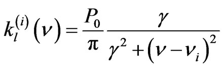
  the contour of the line absorption, i.e. the spectral intensity of the laser impulse;
  the contour of the line of absorption of the studied body;
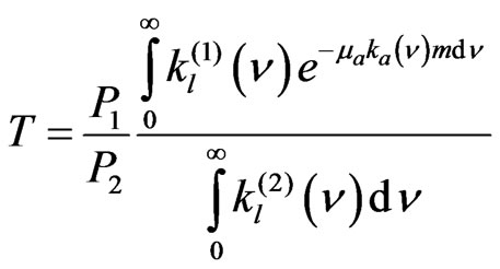
  the spectral coefficient of absorption for the other processes of interaction of the radiation with matter; The power of the laser radiation captured in the hypothesis of homogeneity of the atmosphere [7-9], will express itself then by:
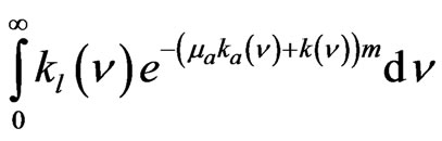 (1)
(1)
where  is the concentration (%) mass (of the component considered in the atmosphere; m: the absorbing matter mass crossed by the laser impulse m = LSρ0, L: the distance the impulse between emitter and the receiving S: area of the surface of the receiving antenna and ρ0 the density of the atmosphere (Figure 2)
 (2)
(2)
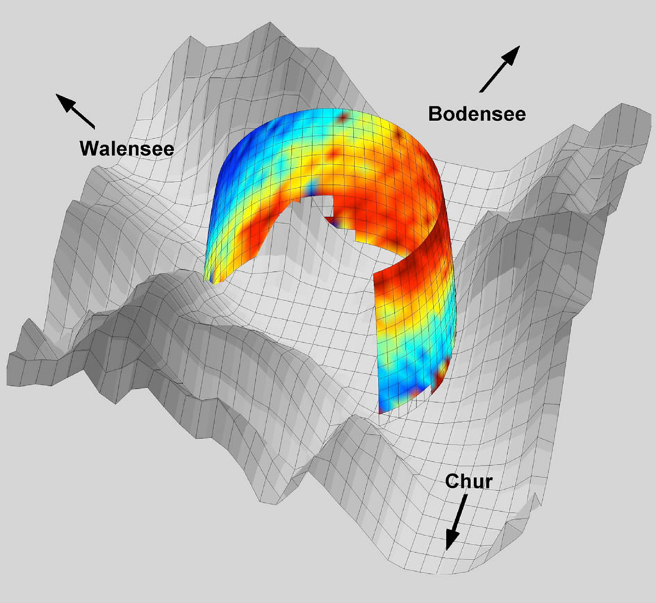

Figure 1. Landscape of a city to quoted of the sea.
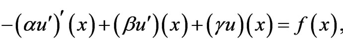
we deal with a simplified model of a coupled transport and Bessel (Figures 3-5) equations.
 (3)
(3)
 (4)
(4)
 (5)
(5)
We can interpret the function transmittance as a wave that has to fulfill the homogeneous wave equation.
 (6)
(6)

 (7)
(7)
When one suppose the following conditions
 ,
,  ,
, 
 , and
, and 

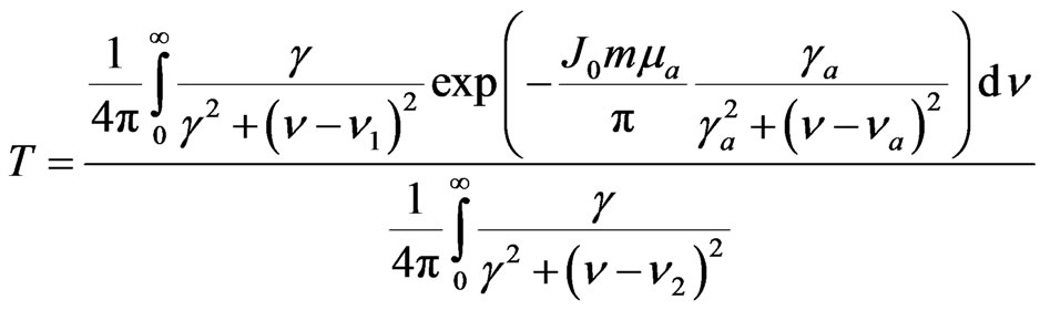
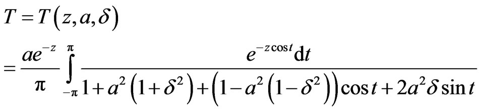
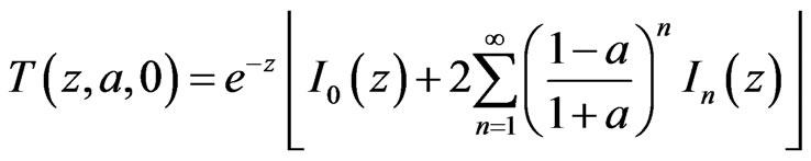
One will be able to write the transmittance:

Figure 2. General case: curve represents the variation of the light intensity in one atmosphere according to the distance.
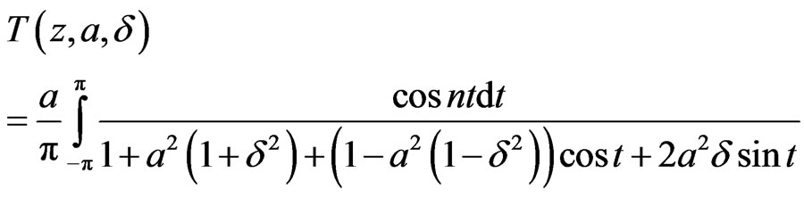 , (8)
, (8)

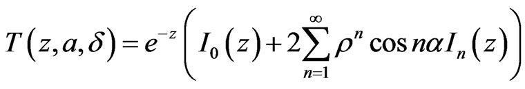
 (9)
(9)
For the left boundaries we have do discretize the following equation:
 (10)
(10)
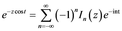
Noticing that ρ < 1 and that for value fixed of z and one has ,
, 
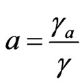
The gotten formulas permit to calculate the function transmission T for values arbitrary of ,
,  ,
,  ,
,  ,
,  ,
,  , as well as to examine some cases different limits. Let’s suppose for example that
 , i.e. that the frequency of the signal confounds itself with the center of the absorption line [10-12]. One then:
 If
If , or
, or 
One has then according to the Equation (10)
In particular, if , one has
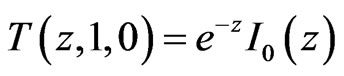
The contribution [Piazzola & all] to coefficient K in inverse kilometers by aerosol particulates can written as
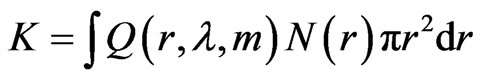 (11)
(11)
We calculate the atmospheric transmission using the expression
 (12)
(12)
The relative variation of the atmospheric transmission is given by
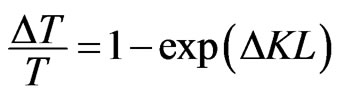 (13)
(13)
3. Simulation Distribution-Diffusion
Before you begin to format your paper, for the 3D dimensional diffusion equation we apply a second order finite difference scheme in space and a higher order discretization scheme in time. We deal with higher order time-discretization methods. Therefore [13-16] we

Figure 3. Transmittance a function of bessel modified.
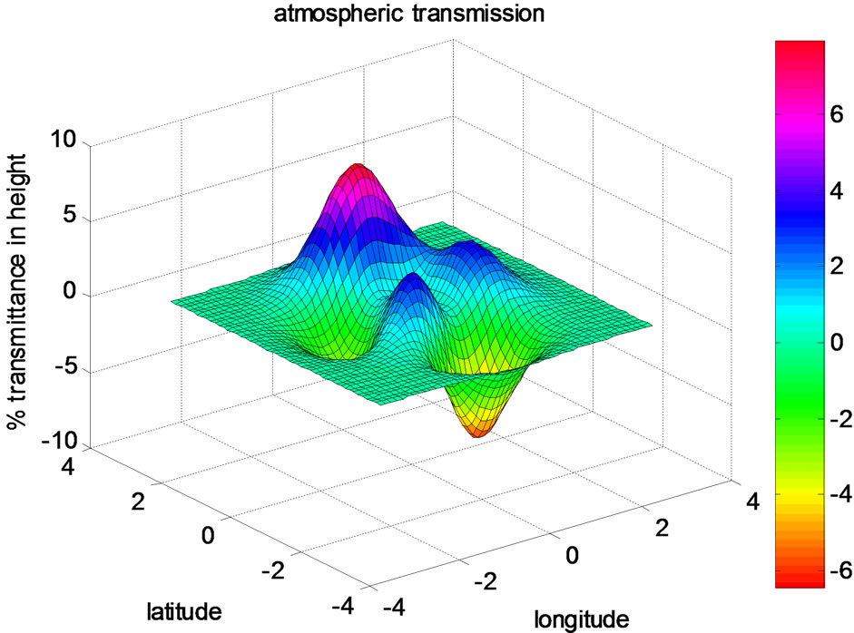
Figure 4. Weak variability spatial and temporal movement.
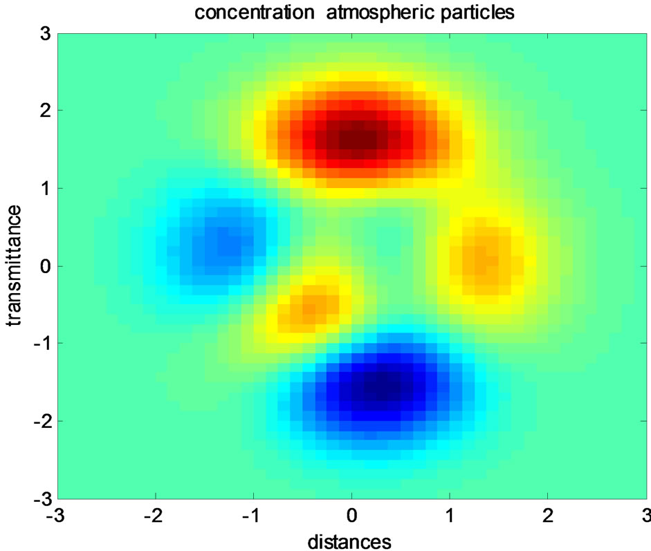
Figure 5. Distributions of pollutants particles.
propose the Runge-Kutta as adapted time-discretization methods to reach higher order results. For the time-discretization we use the following higher order discretization methods (Figures 6-8).
We deal with the following semi-discretized partial differential equations; such equations are used in each iterative splitting step:
 (14)
(14)
where ν is the operator that we implicit solve in the equation and is the explicit operator, with a previous solution, e.g. last iterative solution. One supposes that the total flux  one generalizes the problem (11) under the form:

one approached the calculation with the method of Galerkin non consolidated.
For flexible specification of these model properties, a great number of variables and functions are available. with  = 10 m2/s, β = −0.3 m/s. In the simulations id given by Quartaroni & All [17,18], one took a concentration u0 of 1 particle by m3 a height of 10 km the number of global.
Peclet is therefore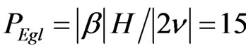 , with
  = 10 m2/s, β = −0.3 m/s. Several examples on the effects of meteorological parameters (i.e., wind velocity, ambient air temperature, atmospheric stability and surface roughness) on pollutant dispersion were illustrated using the program.
4. Conclusions
The aim of this paper was to assess the vertical variations in atmospheric transmission calculated from vertical aerosol concentration profiles recorded in stratospheric

Figure 6. The oscillations of the parasites in function of winds.


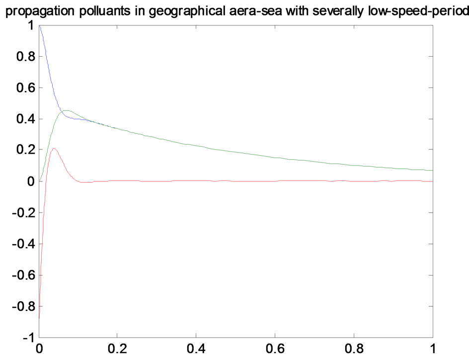
Figure 7. Distributions particles with speed winds.
area. The analysis of the data revealed a negative transmission gradient between 0.3 and 0.4 m height during winds of marine origin lower than 8 m/s, whereas a positive gradient occurs between 0.5 to 0.6 to 0.9 m height during high-wind-speed periods ( > 8 m/s), these distribution particles gradients induce a relative difference in atmospheric transmission between the two sample heights, which is maximal in the 3 - 5 μm band for winds lower 8 m/s, compared to the 8 - 12 μm band.
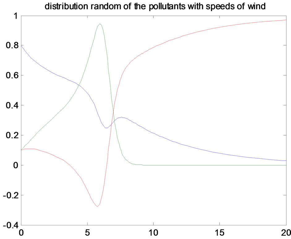
Figure 8. Simulation of the pollutants with random speed winds distributions.
However, comparisons with in situ data show the need for realistic source function and to model the specific situation of the geographical location. The present paper provides a simple approach to the complex problem of the aerosol dynamics during severally seasons. A realistic simulation would take into account a set of the aqueous or gaseous chemistry equations which we have ignored here. This tool is under development in our laboratory, and includes specialized modules: dust/radiation interaction, wet scavenging, an improved dust scheme, and a more detailed emission map for the carbonaceous particles. Finally, the pollutants, emitted once in the atmosphere, can be transported on long distances and to cause some damages in regions relatively faraway of the places of emission.
REFERENCES
- H. Nakatsuka, S. Asaka, H. Itoh, K. Ikeda and M. Matsuoka, “Observation of Bifurcation to Chaos in an Alloptical Bistable System,” Physical Review Letters, Vol. 50, No. 2, 1983, pp. 109-112. doi:10.1103/PhysRevLett.50.109
- K. Tamura, E. P. Ippen, H. A. Haus and L. E. Nelson, “77-fs Pulse Generation from a Stretched-Pulse ModeLocked All-Fiber Ring Laser,” Optics Letters, Vol. 18, No. 13, 1993, pp. 1080-1082. doi:10.1364/OL.18.001080
- G. Yandong, S. Ping and T. Dingyuan, “298 fs Passively Mode-Locked Ring Fiber Soliton Laser,” Microwave and Optical Technology Letters, Vol. 32, No. 5, 2002, pp. 320-333. doi:10.1002/mop.10170
- K. K. Gupta, N. Onodera and M. Hyodo, “Technique to Generate Equal Amplitude, Higher-Order Optical Pulses in Rational Harmonically Mode-locked Fiber Ring Lasers,” Electronics Letters, Vol. 37, No. 15, 2001, pp. 948- 950. doi:10.1049/el:20010584
- Y. Shi, M. Sejka and O. Poulsen, “A Unidirectional Er/sup 3+/-doped Fiber Ring Laser without Isolator,” IEEE Photonics Technology Letters, Vol. 7, No. 3, 1995, pp. 290-292. doi:10.1109/68.372749
- J. M. Oh and D. Lee, “Strong Optical Bistability in a Simple L-Band Tunable Erbium-Doped Fiber Ring Laser,” IEEE Journal of Quantum Electronics, Vol. 40, No. 4, 2004, pp. 374-377. doi:10.1109/JQE.2004.824699
- Q. Mao and J. W. Y. Lit, “L-Band Fiber Laser with Wide Tuning Range bases on Dual-WaveLength Optical Bistability in Linear Overlapping Grating Cavities,” IEEE Journal of Quantum Electronics, Vol. 39, No. 10, 2003, pp. 1252-1259. doi:10.1109/JQE.2003.817239
- L. Luo, T. J. Tee and P. L. Chu, “Bistability of Erbium-Doped Fiber Laser,” Optics Communications, Vol. 146, No. 1-6, 1998, pp. 151-157. doi:10.1016/S0030-4018(97)00502-6
- P. P. Banerjee, “Nonlinear Optics—Theory, Numerical Modeling, and Applications,” Marcel Dekker Inc., New York, 2004.
- P. Meystre, “On the Use of the Mean-Field Theory in Optical Bistability,” Optics Communications, Vol. 26, No. 2, 1978, pp. 277-280. doi:10.1016/0030-4018(78)90071-8
- L. A. Orozco, H. J. Kimble, A. T. Rosenberger, L. A. Lugiato, M. L. Asquini, M. Brambilla and L. M. Narducci, “Single-Mode Instability in Optical Bistability,” Physcal Review A, Vol. 39, No. 3, 1989, pp. 1235-1252. doi:10.1103/PhysRevA.39.1235
- K. Ikeda, “Multiple-Valued Stationary State and Its Instability of the Transmitted Light by a Ring Cavity System,” Optics Communications, Vol. 30, No. 2, 1979, pp. 257- 261. doi:10.1016/0030-4018(79)90090-7
- M. J. Ogorzalek, “Chaos and Complexity in Nonlinear Electronic Circuits,” World Scientific Series on Nonlinear Science Series A, Vol. 22, 1997.
- M. P. Kennedy, “Three Steps to Chaos—Part I: Evolution,” IEEE Transactions on Circuits Systems—I: Fundamental Theory and Applications, Vol. 40, No. 10, 1993, pp. 640-656.
- N. J. Doran and D. Wood, “Nonlinear-Optical Loop Mirror,” Optics Letters, Vol. 13, No. 1, 1988, pp. 56-58. doi:10.1364/OL.13.000056
- S. Zhang, Y. Liu, D. Lenstr, M. T. Hill, H. Ju, G.-D. Khoe and H. J. S. Dorren, “Ring-laser Optical Flip-Flop Memory with Single Active Element,” IEEE Journal of Selected Topics in Quantum Electronics, Vol. 10, No. 5, 2004, pp. 1093-1100.
- M. E. Fermann, F. Haberl, M. Hofer and H. Hochreiter, “Nonlinear Amplifying Loop Mirror,” Optics Letters, Vol. 15, No. 13, 1990, pp. 752-754. doi:10.1364/OL.15.000752
- A. Quarteroni, S. Ricardo and F. Saleri, “Méthodes Numériques: Algorithmes, Analyse et Applications,” Springer, New York, 2008.