American Journal of Molecular Biology
Vol.3 No.1(2013), Article ID:27190,15 pages DOI:10.4236/ajmb.2013.31003
Using Bayesian and Eigen approaches to study spatial genetic structure of Moroccan and Syrian durum wheat landraces
![]()
1ICARDA Office, Rabat, Morocco
2School of Agricultural and Forestry Engineering, Cordoba University, Cordoba, Spain
Email: *m.nachit@cgiar.org
Received 4 June 2012; revised 4 July 2012; accepted 27 August 2012
Keywords: Durum Wheat; Breeding; Landraces; Morocco; Syria; Genetic Structure; Eigenanalysis; Bayesian
ABSTRACT
The Mediterranean durum wheat landraces are genetically diverse and important sources for improving resistance to abiotic and biotic stresses and developing adapted and productive durum wheat varieties in the Mediterranean region. To study the diversity two distant countries (Morocco and Syria) durum landraces were studied. Fifty-one microsatellites were used as molecular markers tool to determine the genetic structure and spatial adaptation of these landraces. We used two spatially-explicit methods (Bayesian and Eigen) to determine the genetic diversity and structure of a population composed of Moroccan (98) and Syrian (90) durum wheat landraces. Non-spatial methods were also applied for comparison. A significant genetic difference was detected between the landraces originated from Morocco and Syria. Six subpopulations were revealed for each country using the Bayesian method and the Eigenanalysis, which generated PC1 and sPC1, showed similar structure. Eigenanalysis exhibited a significant global genetic structure for both countries landraces; and showed that neighboring landraces tend to have close genetic profile. The two first axes of PC1 and sPC1 had discriminated four out of the six subpopulations revealed by the Bayesian methodology. Also, our study detected the close relationship between the durum landraces from the coastal areas of Syria and the Moroccan landraces from the Atlantic coastal regions where the Phoenicians/Carthaginians had settled in Morocco. These results demonstrate the importance of using the spatial models in genetic analysis of durum wheat landraces; and also recommend the use of the easily usable Eigenanalysis to analyze the genetic diversity and structure.
1. INTRODUCTION
Breeding durum wheat for dryland and for the areas which are affected severely by drought and heat and other factors of climatic changes, such as in the Mediterranean region, requires novel genes to be incorporated in future cultivars to cope with these stresses. One of the main objectives of the durum wheat breeding program at the International Center for Agriculture Research in the Dry Areas (ICARDA) is to improve resistance/tolerance to the Mediterranean abiotic and biotic stresses. Our earlier studies have shown that the Mediterranean durum wheat local landraces are important sources for resistance to abiotic and biotic stresses, to develop adapted and productive durum wheat genetic material combining high yield, improved grain quality, and resistance to the stresses, particularly to drought and foliar diseases [1]. The Mediterranean basin is rich in durum wheat landraces and Triticum wild relatives, which are found growing in different agro-ecologies. These Mediterranean landraces possess desirable traits related to resistance to drought, heat, and cold, such as early vigor, long peduncle, and high fertile tillering capacity; and to grain qualities required for different durum wheat end products. In the Eastern Mediterranean basin, Syria is considered as one of the most important habitats for Triticum wild relatives and landraces of durum wheat; and where some landraces are still grown by the farmers such as Haurani and Hamari [2]. Also in the Western Mediterranean basin, Morocco durum wheat landraces are grown in different agro-ecologies, altitudes, latitudes, and water regimes; and carry tolerance/resistance to various abiotic and biotic stresses [1,2]. Multi-allelic microsatellite markers can be employed for the determination of genetic structure and spatial adaptation of these landraces. The allelic variation is critical to the survival of a species and to the adaptation to drought, temperature extremes (cold and heat), and climate changes. The variation is revealed by genetic diversity; where a large gene pool is bound to the ability to survive under stressed conditions. The analysis of the structure of variations is important for breeding purposes, especially to identify genes or genomic regions involved in adaptation to these environmental stresses. Molecular markers and development of statistical techniques to analyze genotypic and phenotypic data have been recently made to study the genetic structure in several species [3]. The genetic structure is necessary for a valid association mapping, because it affects the pattern of linkage disequilibrium [4,5]; and also helps in the detection of candidate genes of interest for breeding [6,7]. For this purpose, several computation programs have been developed [8]. The popular program to detect population structure among individuals is provided by the STRUCTURE program [4], which uses the Bayesian clustering method. The general principal of Bayesian method considers data and parameters as random variables [9]. These random variables have a joint distribution, called a-priori. Bayesian statistics aims manipulating the joint distribution in various ways to infer the parameters. Bayesian inference calculates the posterior distribution of parameters, which is the conditional distribution of parameters given the data [9]. Moreover, in the last decade, there is increasing evidence that genetic diversity is mediated by space [10]. The geographical dimension (space) of genetic process uses space to display graphically results from genetic analysis and ordination methods [11]; and to compute spatial autocorrelation [12-15]. All these methods may reveal and quantify spatial pattern of genetic data, but they are not explicit. To be explicit, a method should include space into analysis, in order to adjust the model used. In 2002, Dupanloup et al. [16] developed the spatial analysis of molecular variance; in 2005, Guillot et al. [17] the GENELAND; and in 2006, François et al. [18] the hierarchical Markov random field (HMRF) model. The last two programs were proposed as an improvement of the STRUCTURE program, they integrate geographic information to infer the number of populations and detect the genetic discontinuities among these populations [19]. Other valid methods are the classical multivariate analyses, such as clustering or Eigenanalysis. An Eigenanalysis is a mathematical operation on a square symmetric matrix, and is therefore central for linear algebra. The output of an Eigenanalysis consists of a series of eigenvalues and eigenvectors (each eigenvalue corresponding to an eigenvector). Principal Component Analysis (PCA) and Correspondence Analysis (CA) are Eigenanalysis.
One of the most used Eigeanalysis methods to investigate structure is the principal components analysis (PCA) according to Cavalli-Sforza [20]. The PCA reduces space scale and its utilization is not contingent on a particular genetic model; therefore Hardy-Weinberg equilibrium or linkage equilibrium are not required for the analysis. PCA is useful to infer and test the number of subpopulations/groups represented in a set of genotypes using Tracy-Widom test [21] and to correct for population stratification in trait-marker association [22]. A new tool for spatial pattern of genetic variability was developed by Jombart et al. [23] called spatial principal components analysis (sPCA). The sPCA is a modified PCA to study the genetic variance between individuals taking into account spatial autocorrelation of allele frequencies.
Few studies were conducted on detailed population structure in durum wheat landraces. Our earlier work [24] studied genetic diversity and measured genetic distance between durum wheat cultivars and some landraces of diverse eco-geographical origin using Restriction Fragment Length Polymorphism (RFLP). Further, Maccaferri et al. [25] have studied the structure and Linkage Disequilibrium (LD) of an elite collection of durum wheat using STRUCTURE and TASSEL programs. Unweighted Pair Group Method with Arithmetic Mean (UPGMA) was used to separate white glumes, black awned, black glumes, and white awned, and classified wheat-like accessions among 56 accessions of durum wheat using SSRs [26]. High and low molecular weight glutenin and clustering method were used by Moraguees [27] to study the genetic diversity between 63 Mediterranean durum wheat landraces. Zarkti et al. (2010) measured genetic distance and diversity of 23 Moroccan durum wheat accessions of which 17 were landraces and using 7 SSRs; and assumed that the genetic variability found in durum wheat may be due to anthropogenic, geographical or environmental effects [28]. The present study aims to 1) determine the genetic diversity and the structure of the Moroccan and Syrian durum wheat landraces using a large set of microsatellite markers covering the whole genome of durum wheat; and 2) to analyze the data with the spatially-explicit Bayesian-based clustering method (GENELAND) and the Eigenanalysis (PCA and sPCA).
2. MATERIAL & METHODS
2.1. Plant Material
The plant material consisted of 98 durum wheat landraces from Morocco collected in 1985; and 90 from Syria collected in 1987 by the ICARDA Genetic Resources Unit (GRU). The landraces cover the main durum wheat agro-ecological zones of the two countries, for Morocco see Figure 1(a)) and for Syria see Figure 1(b)). The
 (a)
(a)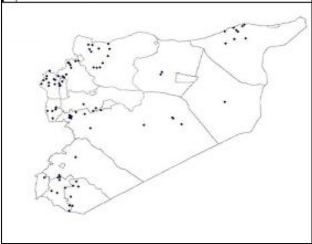 (b)
(b)
Figure 1. Spatial distribution of the Moroccan (a) and Syrian (b) durum landraces.
spatial coordinates (latitude, longitude, and altitude) were recorded. The two collections were genotyped at the ICARDA durum wheat-breeding program, using 51 Gatersleben wheat microsatellites (gwm) covering all the 14 chromosomes of the durum wheat genome (Table 1). Alleles were attributed according to the fragments size in base pair (bp). In this study, we analyzed three datasets: The combined dataset from both countries containing the 188 landraces (population structure, spatial population structure, PCA and sPCA); and the separate dataset for each country (spatial population structure, PCA and sPCA).
2.2. Descriptive Locus Statistics
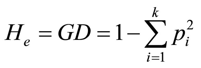
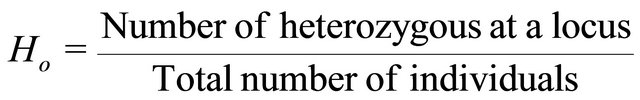
In this study, we computed for each SSR locus and each population the following parameters using a program developed with Visual Basic for Application under Excel: Expected heterozygosity (He) or genetic diversity (GD) estimates the fraction of all landraces which would be heterozygote for any randomly chosen locus and is calculated as:
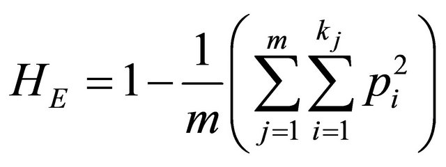
 where pi is the frequency of the ith allele and k is the total number of alleles of the studied locus. The expected heterozygosity over m loci (HE) is:
 .
.
Observed heterozygosity (Ho) of a population is measured by determining the proportion of loci that are heterozygote and the number of landraces that are het-
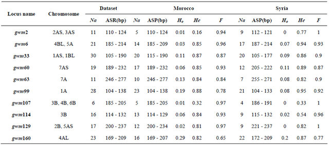
Table 1. Locus descriptive parameters for the Dataset and for the Moroccan and the Syrian durum wheat landraces populations.
Continued
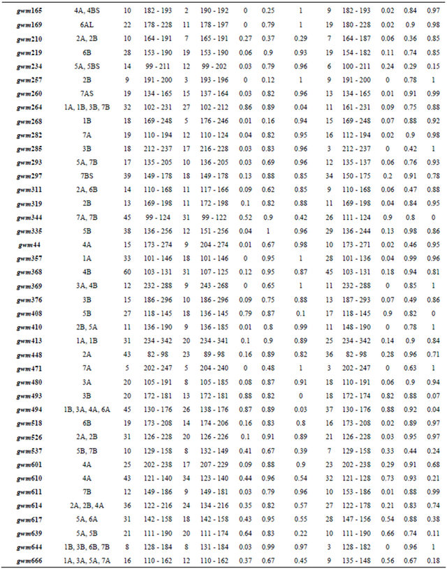
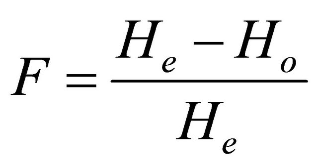
Abbreviations. Na: The number of observed alleles by loci. ASR (bp): Allele size range in base pair. Ho: Observed heterozygosity. He: Expected heterozygosity. F: The inbreeding coefficient.
erozygote for each particular locus. For a single locus with two alleles, Ho is defined by:
 .
.
Over a series of several loci, Ho is the sum of Ho calculated for each locus divided by the number of considered loci. Wright [29] developed F-statistics as measures of genetic structure. For a locus, F is defined as:
 .
.
F has values between 0 for no genetic drift; and 1 fixation of alternative alleles.
2.3. Bayesian Genetic Structure
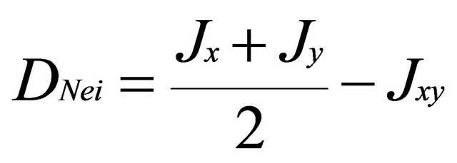
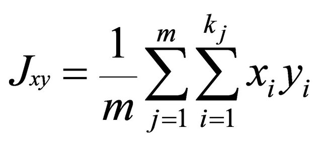
We examined the genetic structure using the spatial model of GENELAND [17,30-32]. Structure was also used as a non-spatially-explicit method for comparison. The main difference between spatial and non-spatial methods is the consideration of the a priori distribution used in Bayesian statistics. While in STRUCTURE the a priori distribution is uniform through the studied space, in GENELAND, it is randomly modeled across space, using Poisson-Voronoi tessellation model. This model assumes that there is an unknown number of polygons that approximate the true pattern of population spread across space [30]. Markov Chain Monte Carlo (MCMC) simulation is used to infer these parameters and to estimate the posterior probability that the data fits the hypothesis of K populations [30]. For both programs, we tested values of K ranging from 2 to 8 with 3 independent runs per test, using no admixture model with correlated allele frequencies [33], a 100,000 iterations burn-in followed by 106 additional iterations, from which every 100th observation was recorded. The spatial studied domain in both countries was divided into a grid of 2500 pixels and GENELAND calculates the posterior probability of every pixel and landrace to belong to a specific cluster (population). In addition, we used Nei’s minimum genetic distance [34] to compute genetic distance between subpopulations from the two countries:
 where xij and yij are the frequencies of allele i at locus j for population x and y, kj is the number of alleles at locus j, m is the number of evaluated loci.
 .
.
2.4. Principal Component Analysis for Multi-Locus Data
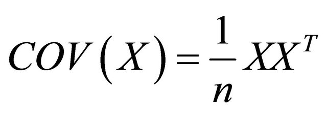
Principal component analysis (PCA) on molecular data is based on the matrix of allelic frequencies for populations or individuals; which considers rectangular matrix C(n, m) with rows indexed by n individuals or populations and columns by m allele frequencies. In the case of the durum wheat landraces data probed with microsatellites, the values composing C are 2 for homozygote landrace, 1 for heterozygote landrace, and 0 for no data. The matrix C is used for PCA analysis under two forms: normalized or not. The normalization can be done using the mean µ(j) and standard deviation σ(j) of each column j of C:
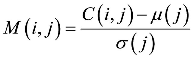 .
.
The common method to visualize PCA results is to plot one eigenvector against another. Geographic coordinates for landraces or populations can be used to produce a contour or heat map using spatial interpolation technologies found at any mapping software to show how an eigenvector varies across space. Also, the test for the spatial autocorrelation of the PCA axes to assess the signifycance of spatial pattern of molecular data was generated. The PCA analysis was conducted using the “ade4” package developed under R [35] (R Development Core Team 2008) by Dray and Dufour [36].
2.5. Spatial Principal Component Analysis
We used the spatial principal component analysis (sPCA) to study the spatial population structure. As for PCA analysis, this method requires no assumption on HardyWeinberg or linkage equilibrium and does not assign landraces to discrete subpopulations. Jombart [37] implemented it under R. This is a “spatially explicit multivariate method” that accounts for genetic variability and spatial structure. The use of sPCA aimed to analyze the studied set of durum wheat landraces allelic frequencies, in order to determine the genetic variability and to reveal the existing spatial patterns. The spatial information is incorporated in the analysis using a spatial weighting matrix w (wij, i = 1 to n, j = 1 to n, n is the number of locations) to describe spatial dependency between landraces. If the location of landrace i is adjacent to the location of landrace j, the weight receives, for example, 1 and 0 if not. This matrix is more often a result of a spatial connectivity network [38]. A spatial connectivity network is a graph constructed in Euclidean space and used to quantify the physical interconnectivity of n landraces within space. The connection between nodes depends on their spatial distance and in general taking place between nearest landraces. The basic element of sPCA method is the spatial autocorrelation (SAU) under the form of Moran’s I [39,40]. The Moran’s I of a vector of allelic frequencies x of n landraces is:
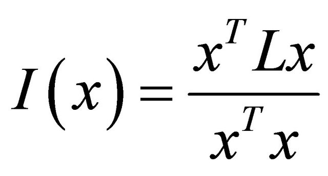 where L the standardized matrix of the weighting matrix w. L is row-standardized (each of its rows sums to 1 with diagonal values are 0). The values of Moran’s I range from +1 meaning strong positive SAU, to 0 meaning a random pattern to −1 indicating strong negative SAU. While the solution of PCA problem is to find eigenvalues of
 the sPCA define a criterion function
 .
.
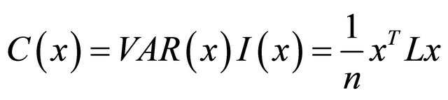
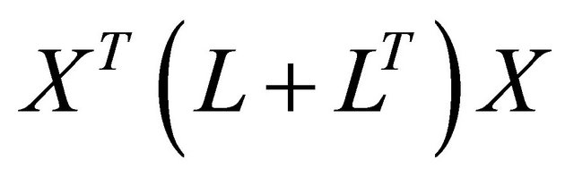
This function measures both spatial structure and the variability of the allelic frequency vector x. C(x) is highly positive when x has a large variance and a positive SAU (global structure); and C(x) is highly negative when x has a large variance and a negative SAU (local structure). This function is the criterion used in sPCA. For X(n, m) composed by m allelic frequencies vectors of n landraces, the solution of sPCA is then giving by finding the maximum and minimum of the criterion function C. These max and min values are found by the eigenvalue decomposition of
 .
.
At the opposite of PCA analysis, eigenvalues of sPCA can be positive or negative for global or local structure respectively. Global scores can identify subpopulations or groups of individuals that are genetically similar and local scores can discriminate between neighboring individuals. To perform sPCA analysis, we used “adegent” package [37]. The test for global and local structure was executed using Monte Carlo test, implemented in the same package, using 106 permutations. A t-test to evaluate if the axes PC1, PC2, PC3 and sPC1 resulting from the Eigenanalysis can discriminate between the subpopulations found by GENELAND was computed using Genstat [41] for Windows.
3. RESULTS
3.1. The Combined Moroccan/Syrian Durum Wheat Landraces Dataset
The total number of amplified alleles of the probed 51 microsatellites loci for the 188 landraces was 1208 alleles. The number of alleles per locus ranged from 5 for gwm471 to 60 for gwm368. The number of alleles per locus was higher in the Syrian landraces (28 loci) than in the Moroccan ones and equal in 4 loci. Almost 50% of locus showed a high value of heterozygosity for the Syrian than the Moroccan durum population. The marker with the highest heterozygous proportion was gwm494; and the lowest gwm257 (Table 1). For the genetic diversity, the expected heterozygosity was significantly (p < 0.001) higher than the observed one, with a mean of difference of 0.56. The non spatial Bayesian method (Structure) analysis separates clearly between the Moroccan and the Syrian durum landraces. However, 16 landraces from the coastal areas of Syria were grouped with the Moroccan landraces population; and one landrace (Sherieh) was assigned equally to both populations. These results indicate that durum wheat in North Africa may have been introduced from the coastal areas of the Middle East where the Phoenicians had lived and later immigrated to the Western Mediterranean countries. This is supported by the strong relationship found in this study between the coastal durum wheat landraces from Syria and the Moroccan ones. Furthermore, landraces from the far south of Morocco, ICDW20038-Tiznit and ICDW 20041-Tiznit were grouped with the Syrian coastal area populations (Figure 2(a)), suggesting that the durum wheat advanced from the coastal areas to South and East of Morocco. In the spatial Bayesian methods (GENELAND) analysis using 106 iterations, at 85% runs the number of populations detected was 2; and the remaining 15% runs detected 3 populations. Distinction between the two populations was clearly shown if the number of populations K = 2 is considered (Figure 2(b)). When we consider K = 3, the third subpopulation is composed by 19 landraces (16 from Syria and 3 from Morocco). This results suggest that our landraces population belong at 85% to one or the other country using the GENELAND program. This is due mainly to the fact that the two countries are geographically distant. As for the PCA analysis, the two first eigenvalues explained 6% of the total variance and plotting the first axis against the second axis demonstrated clear evidence for the structure and for the difference between the two durum landraces populations (Moroccan and Syrian) especially the first axis, which was positive for the Moroccan landraces and negative for the Syrian ones. Using the t-test, the means of the first axis significantly differ between the Syrian population and the Moroccan one (p < 0.001). However, the Syrian coastal landraces formed the exceptions found at STRUCTURE results and showed similarity to the Moroccan landraces (Figure 2(c)). The sPCA analysis gave similar results as the previous analysis with approximately the same exceptions for the similarity be-
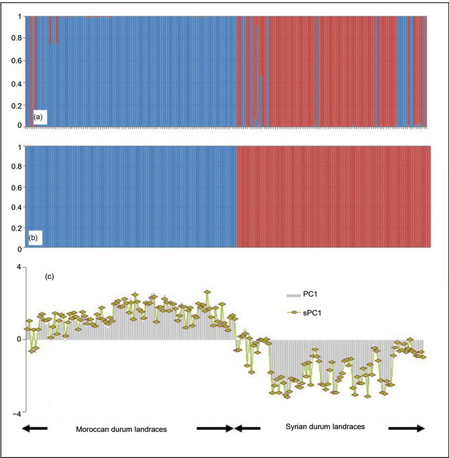
Figure 2. Genetic structure of the Moroccan and Syrian durum wheat landraces. (a) STRUCTURE chart; (b) GENELAND chart; (c) first principal component PC1 (Grey bars) and first spatial principal component sPC1 (Green points).
tween Syrian coastal landraces and Moroccan landraces (Figure 2(c)). We used for sPCA a minimum distance connection network, in order to disconnect Syrian and Moroccan landraces imaging the spatial geographical distance.
Correlation between PC1 and sPC1 coordinates was very highly significant (p < 0.001) with an R2 of 98%. A correlation with groups between the two axes and using the landraces origin as factor was also highly significant (p < 0.001) with a coefficient of 0.98.
3.2. Moroccan Durum Wheat Landraces Population
We observed 741 alleles in the Moroccan population using 51 microsatellites. For the range, the highest value was scored with 34 alleles at the locus gwm610; and the lowest with 2 alleles at gwm165. The average per locus was 14 alleles. Six of the studied markers were 100% homozygote (gwm357, gwm169, gwm369, gwm471, gwm165, gwm257) and 3 were higher than 80% heterozygote (gwm493, gwm494, gwm264). Expected het erozygosity ranged from 0.99 for gwm335 and gwm644 to 0.11 for gwm257; and HE was 0.763 (Table 1). He was significantly (p < 0.001) higher that Ho and with a mean difference of 0.5. GENELAND estimated six Moroccan sub-populations at 95%, five at 3% and four at 2%. The degree of inclusion to a subpopulation of most landraces was more than 90% (Figure 3(a)). Maps of posterior probabilities of the six subpopulations are shown in Figure 4; and were named P1M, P2M, P3M, P4M, P5M and P6M. Eleven landraces were attributed at more than 90%
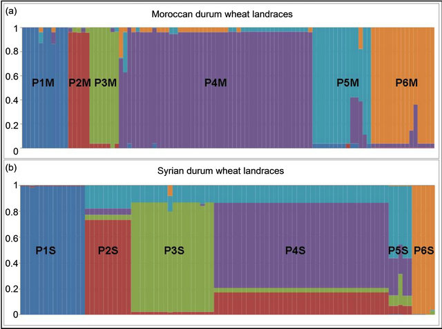
Figure 3. GENELAND chart for the six Moroccan (a) and Syrian (b) subpopulations.
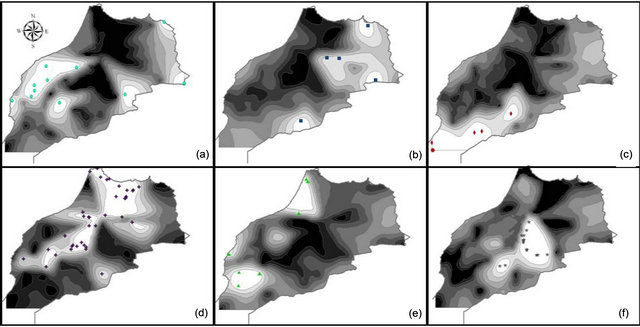
Figure 4. Moroccan landraces population probability assignments on the Morocco studied area (high probability: white; low probability: dark). (a) P1M, (b) P2M, (c) P3M, (d) P4M, (e) P5M and (f) P6M.
to the subpopulation 1 (P1M), 7 of them are from Tensift and two from Doukala regions (South Casablanca-Marrakech region), region that is influenced by the Atlantic ocean, but this subpopulation contains as well 3 other landraces from the North-Eastern region of Oujda and Figuig, which is also influenced by the Mediterranean Sea. P1M represents the semi-arid and maritime (SAM). The second subpopulation (P2M) was attributed at 96%; and contains 2 landraces originated from the irrigated areas of the South-Eastern Atlas high plateaus and 3 landraces from the highlands of Boulman and Nador regions in the eastern plateaus of Middle-Atlas and Rif Mountains. P2M represents the arid and cold plateaus (ACP). The third subpopulation (P3M) consists of 8 landraces from southern warm areas of Morocco (Tata, Tiznit, Goulmine). P3M represents the arid and maritime areas (AM). As for the subpopulation (P4M), it has the largest number of landraces (46). The landraces of the P4M cluster are originated mainly from the western mountainous cold areas of the Atlas Mountains and Rif chains; P4M represents the rainfall-favorable high altitude-cold areas (RFHAC). Furthermore, most of the 14 landraces of subpopulation 5 (P5M) were originated from the southern Atlantic lowland region of Morocco (Taroudant, Agadir, and Essaouira. P5M represents the irrigated/rainfall-favorable maritime areas (IRFM); and 3 landraces from the northern Atlantic lowland region (Larache), representing the maritime high rainfall areas. These latter ones were assigned as well to P4M at 40%. The sixth subpopulation (P6M) had 15 landraces from Moroccan pre-and anti-Atlas areas (Beni Mellal, Khenifra, Errachidia and Ouarzazate), P6M represents the irrigated continental/cold plateaus (ICCP) of the pre-and anti-Atlas plateaus of South-East Morocco. The results divided clearly the landraces originating from environmentally water stressed and non-stressed regions of Morocco; with P1M, P2M, and P3M for the stressed and P4M, P5M, and P6M for the non-stressed conditions. The heterozygozity, the number of alleles, the individuals, and the agro-ecological regions of collection of landraces composing each subpopulation are summarized in Table 2.
P2M, P3M, and P5M found in the Eastern and Southern parts of Morocco had the largest number of alleles per locus and the large values for heterozygosity compared with P4M of the highland areas. The P4M had on the other hand, the lowest number of homozygote loci. We used the matrix of allele frequencies without standardization for PCA analysis. The first three eigenvalues were 52.23, 11.75, and 4.78 explaining 30.9%, 7.0%, and 2.9% of the total genetic variability, respectively. The corresponding axes are symbolized PC1, PC2 and PC3 in this study. In the sPCA analysis, we used Gabriel graph as spatial connecting network. The spatial autocorrelation (SAU), under the form of Moran’s I, applied to allele frequencies showed that 30% of the alleles showed no SAU with a value of I = I0 = −0.01. Eighty alleles had a significant positive SAU with a maximum value of 0.43 observed at the allele gwm282.217. The first (λ1) and the last (λ97) eigenvalues had the strongest variance with positive SAU value for λ1 and negative for λ97. The global and local tests presented by Jombart et al. (2008) showed a significant global test (p = 0.02) and non-significant local test (p = 0.26). Therefore, only the global structure is significant and then only λ1 is interpretable in the case of the Moroccan landraces; conesquently, only the first sPCA axis, the sPC1 is considered. The SAU for sPC1 was 0.47, PC1: 0.28, PC2: −0.02 and PC3:0.27. This means a global structure is given by PC1 and PC3. In addition to the positive value of SAU of PC1
Table 2. Moroccan durum wheat subpopulations genetic information.

Ho is the observed heterozygosity and He is the genetic diversity.
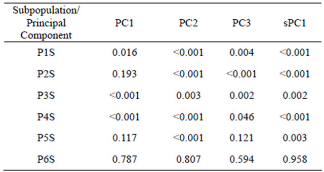
and sPC1, mapping PC1 and sPC1 over the studied areas of Morocco showed a very strong visual spatial pattern schematized by a positive component for landraces from the high altitude (Rif and Atlas mountains) landraces and a negative component elsewhere (Figure 5). In general, neighboring landraces had close coordinates on the PC1 and sPC1 axes. Correlation between PC1 and sPC1 coordinates was very highly significant (p < 0.001) with a coefficient of 0.87. A correlation between the two axes and using subpopulations found by GENELAND, as factor was also highly significant (p < 0.001) with a coefficient of 0.61. The t-test (Table 3) showed that only P2M could not be differentiated by the four axes (sPC1, PC1, PC2 and PC3). sPC1 and PC1 discriminated clearly between 4 out of the six Moroccan subpopulations detected by GENELAND.
3.3. Syrian Durum Wheat Landraces Population
The number of observed alleles was 836 with a maximum of 45 alleles for the locus gwm368 and with a minimum of 3 alleles for gwm471, gwm644 and gwm285. Average number of alleles per locus was 16. The molecular markers gwm369, gwm471, gwm257, gwm410, gwm129, gwm644, gwm107, gwm285, and gwm2 were homozygote (100%); whereas gwm493, gwm494, gwm344 and gwm408 were the most heterozygote. As for genetic diversity, values ranged from 0.99 for gwm357 to 0.28 for gwm234 (Table 1). The genetic diversity over all loci was 0.79. The expected heterozygosity was significantly greater than the observed one, with a p < 0.001 and a mean difference of 0.52. GENELAND analysis generated six subpopulations for the Syrian landraces at 88% and five sub-populations at 12% (Figure 3(b)) and inferred posterior probabilities for each of the 2500 pixel of Syrian area belonging to these subpopulations (Figure 6). Only 20 Syrian durum landraces were attributed to a
Table 3. T-test value for subpopulations detected in Moroccan durum wheat landraces.
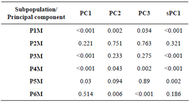
PC1, PC2, and PC3: first, second, and third principal component, respectively. sPC1 is the first spatial component. P1M, P2M, P3M, P4M, P5M, and P6M are the six Moroccan subpopulations detected by GENELAND software.
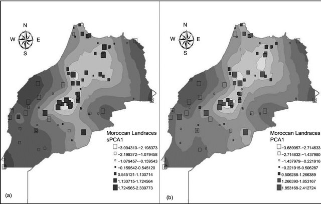
Figure 5. Maps of the first spatial principal (a) and principal (b) components for the Moroccan durum wheat landraces.
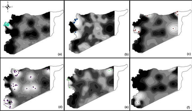
Figure 6. Syrian landraces population probability assignments on the Syria studied area. (a) P1S, (b) P2S, (c) P3S, (d)P4S, (e) P5S and (f) P6S.
population at more than 90%. Subpopulation1 (P1S) was clearly separated from other subpopulations and it was composed of 14 landraces represented mainly by the landraces: Haririe, Sourie, Souedie, which are originated from the coastal Mediterranean region of Syria (Latakia, Elghab and Alhafa). The P1S represents the rainfall-favorable/maritime areas (RFM). Ten landraces were assigned at 71% to the subpopulation2 (P2S) but also to subpopulation 5 (P5S) at 17%. Nine of the landraces were Souedie, and originated from the northeast of Latakia province, in addition to the landrace “Hamari” from Homs province. The P2S represents the rainfall-favorable/high altitude areas (RFHA). The subpopulation 3 (P3S) was the most diversified as inferred by GENELAND, according to the origin of landraces, but also to their nomenclature. They were mainly collected from the Northeast of Syria (Kamishli, Hassakeh and Ras Elayn); however, the third subpopulation (P3S) included also landraces from the coastal western part of Syria (Dreikesh, Tartous and Sheikh Badr), Haurani from Albab near Aleppo and Biadi from Deir Ezzour were also designated to this population. This subpopulation (P3S) is representing the high rainfall /irrigated/semi-continental areas (HRISC); with a percentage of inclusion up to 84%; the remaining landraces were also affected at 13% to population 5 (P5S). The largest subpopulation from Syria was P4S with 38 landraces. Fourteen (14) were “Haurani”, 9 “Baladi”, 9 “Biadi” and 2 “Hamari”. P4S had most landraces originated from the Syrian central NorthSouth axis (Aleppo in the North to Qunaytera in the Golan Heights). The P4S represents the semi-arid continenttal areas (SAC); some of landraces of P4S were also included in P5S at 13%. The fifth subpopulation P5S was difficult to differentiate from the other subpopulations (Figure 3(b)). Five (5) landraces (Baladi from Latakia, Hamari from Safita, Shihani from Hassakeh, Sourie from Alhafa, and Shihani Kandahari from Hassakeh) were inferred to this subpopulation with 50% and shared with P4S at 30%. This subpopulation mainly represents the high altitude/continental/high rainfall areas (HACHR). The last subpopulation P6S is composed by 5 landraces and included two landraces from Ras Alayn, two from Assanamayn, and one from Alqutayfa close to Damascus with inference at 99%. The P6S represents the arid-continetal Areas of Syria (AC). A summary for the six Syrian subpopulations is shown in Table 4. As it was indicated earlier, P4S contains the largest number of landraces, but shows the smallest number of alleles per locus. P3S containing landraces from distant geographical areas but with similar moisture levels through rainfall or irrigation and temperatures (Tartous, Homs, Hassakeh, and Deir Ezzour) was the population with the largest heterozygosity over all loci. As indicated earlier, the P3S is most diversified population; it has the lowest number of homozygote loci compared with the other subpopulations in Syria. Generally, the Syrian durum landraces are found to be grown in different agro-ecologies; i.e. the same landrace is cultivated in different environments, in contrast to the Moroccan landraces, where geographical barriers are more prevailing than in Syria. In the PCA analysis based on the matrix of allele frequencies without standardization, the first three eigenvalues explained 37% of the total genetic variability. The axes are symbolized PC1, PC2, and PC3. Moran’s I index computed for alleles frequencies for the Syrian landraces showed a high SAU (≥0.5) for 8 alleles. However, only 18 had a positive significant SAU. A maximum I of 0.89 was registered for the allele gwm264.169, while 80 alleles showed no significant SAU with a value of I = I0 = −0.01.
On the other hand, 3 alleles gwm293.168, gwm494.191 and gwm666.100 showed significant negative SAU of −0.11, −0.4, and −0.55, respectively. Further, almost 50% of studied alleles had no significant SAU, indicating a random distribution over Syria. As for sPC analysis, we constructed a spatial network with Gabriel graph. Only the global structure was taken into account and it has been differentiated from other eigenvalues (p < 0.001), while the local test was not significant. Therefore, only the first axis (sPC1) is interpretable. PC1 and sPC1 showed almost the same spatial pattern over the studied area of Syria (Figure 7). However, the global spatial pattern was less obvious than in the Moroccan case, as
Table 4. Syrian durum wheat subpopulations genetic information.

Ho is the observed heterozygosity and He is the genetic diversity.
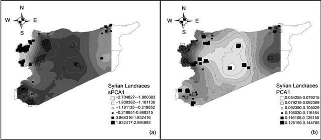
Figure 7. Maps of the first spatial principal (a) and principal (b) components for the Syrian durum wheat landraces.
several neighbor landraces had diverse values for PC1 or sPC1. This is because several alleles showed negative SAU in the Syrian population, and additionally, the number of alleles with significant positive SAU was less present than in the Moroccan landraces population. Using t-test analysis (Table 5), the P6S could not be differentiated from the other five subpopulations by the four axes PC1, PC2, PC3 and sPC1. Furthermore, the sPC1 permitted to discriminate significantly between the first five subpopulations compared with three subpopulations for PC1 that was generated by GENELAND. Correlation between PC1 and sPC1 coordinates was very highly significant (p < 0.001) with a coefficient of −0.73. A correlation between the two axes using subpopulations found by GENELAND, as factor was also highly significant (p < 0.001) with a coefficient of −0.78.
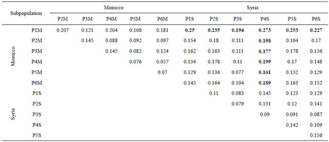
The Nei’s minimum genetic distance (Table 6) showed that the Moroccan subpopulation P1M from the semi-arid and maritime areas was the most distant genetically to all the subpopulations from Syria. Similarly
Table 5. T-test table for populations detected in the Syrian durum wheat landraces.
the Syrian subpopulation P4S from semi-arid and continental areas, was the most distant genetically to all the Moroccan subpopulations. As for the nearest genetically among the subpopulations of the two countries, P3S from the Syrian high rainfall/irrigated/semi-continental areas (Figure 6(c)) was the most nearest to the Moroccan subpopulations, particularly to P5M (Figure 4(e)) from the Atlantic Northwest and coastal areas of Morocco (irrigated/rainfall-favorable/maritime areas), mainly where the Phoenicians had settled. The early center of Phoenician/Carthagians settlements in Morocco (http://www.phoenician.org/phoenician_colonies.htm) were Lixis (Larache), Tingis (Tangiers), Sala (RabatSalé), Zili (Asilah), and Mogador (Essaouira); and these areas are congruent with the prsence of subpopulation (P5M), which is genetically closed to the Syrian subpopulation (P3S) from Syria (Tartous). Within Morocco, the genetically nearest subpopulations were P4M (rainfall-favorable/high altitude-cold areas) and P6M (irrigated continental/cold Atlas plateaus). As for the subpopulations of Syria, the genetically nearest were P2S (rainfall-favorable/high altitude areas) and P3S (high rainfall/irrigated/semi-continental areas).
4. DISCUSSIONS
We showed that similar spatial genetic patterns were found using the two approaches (Bayesian and Eigen) especially for the Moroccan population. The axis of the Eigenanalysis differentiated clearly between clusters revealed by the Bayesian method. The Eigenanalysis is easy to implement, has no assumption on data, and can help in understanding diversity and structure of a given population. The resulting axes are continuous and can be
Table 6. Nei’s genetic distance for the Moroccan and Syrian durum wheat subpopulations.
P = Subpopulation; M = Morocco, S = Syria.
used to correct phenotype trait and genotypic data for association studies [22]. This study showed clearly the geographic distribution of landraces in Morocco and Syria and confirmed that in general, landraces tended to group according not to their geographical origin [27], but also to their agro-ecological adaptation. The use of spatial genetic structure helped largely to understand the mechanisms of adaptation of durum wheat landraces; and that environment (topography, landscape) has a considerable effect on population structure [19]. A detailed analysis of genetic discontinuities through barriers using Monmonier’s algorithm [42,43] may be needed for the association between the durum wheat germplasm genetic discontinuities and environmental barriers. These analyses techniques, aided by marker-trait association, are a powerful tool in the hand of the breeders for deciding on the choice of the parental material in a crossing program [3,27,28]. The amplified alleles found in this study were more than twice than the durum wheat elite collection population [25]. This may be explained that our populations consisted of diverse landraces; whereas the mentioned previous work was mainly of improved genotypes. The genetic diversity found in the Moroccan and Syrian landraces was higher than the diversity found by Moragues and colleagues [27] for a group of Mediterranean durum landraces using low and high molecular weight loci. Moroccan and Syrian durum wheat landraces hold large genetic variability and considerable number of alleles with the probability of having some of these alleles associated with stress tolerance, yield, and/or grain quality [1,2]. The spatial autocorrelation (SAU) applied to an individual allele did not express the global spatial structure we have in our data [15]. Therefore, SAU applied to one specific allele (example of an allele in association with a trait of interest) can be used to investigate the spatial distribution and the correlation of this allele with environmental and/or geographic variables [3].
5. ACKNOWLEDGEMENTS
We are thankful for the helpful discussions and reviews by A. Amri and J. Ryan. The authors also thank the ICARDA durum wheat breeding group, especially Hani Hazzam and Mohammad Alazrak for the field work, and Ahmad Alsaleh for the assistance in genotyping.
REFERENCES
- Nachit, M.M. and Elouafi, I. (2004) Durum adaptation in the Mediterranean dryland: Breeding, stress physiology, and molecular markers. Challenges and strategies for dryland agriculture. CSSA Special Publication 32, Crop Science Society of America Inc., American Society of Agronomy Inc., Madison, 2004, 203-218.
- Pagnotta, M.A., Impiglia, A., Tanzarella, O.A., Nachit, M.M. and Porceddu, E. (2004) Genetic variation of the durum wheat landrace Haurani from different agro-ecological regions. Genetic Resources and Crop Evolution, 51, 863-869. doi:10.1007/s10722-005-0775-1
- Castillo, A., Dorado, G., Feuillet, C., Sourdille, P. and Hernandez, P. (2010) Genetic structure and ecogeographical adaptation in wild barley (Hordeum chilense Roemer and Schultes) as revealed by microsatellite markers. Plant Biology, 10-266.
- Pritchard, J.K., Stephens, M. and Donnelly, P. (2000) Inference of population structure using multilocus genotype data. Genetics, 155, 945-959.
- Flint-Garcia, S.A., Thornsberry, J.M. and Buckler, E.S. (2003) Structure of linkage disequilibrium in plants. Annual Review of Plant Biology, 54, 357-374. doi:10.1146/annurev.arplant.54.031902.134907
- Aranzana, M.J., Kim, S. and Zhao, K., et al. (2005) Genome-wide association mapping in Arabidopsis identifies previously knowing flowering time and pathogen resistance gene. PLOS Genetics, 5, e60. doi:10.1371/journal.pgen.0010060
- Mackay, L. and Powell, W. (2006) Methods for linkage disequilibrium mapping in crops. Trends in Plant Science, 12, 57-63. doi:10.1016/j.tplants.2006.12.001
- Excoffier, L. and Heckel, G. (2006) Computer programs for population genetics data analysis: A survival guide. Nature Reviews Genetics, 7, 745-758. doi:10.1038/nrg1904
- Beaumont, M.A. and Rannala, B. (2004) The Bayesian revolution in genetics. Nature Reviews Genetics, 5, 251- 261. doi:10.1038/nrg1318
- Manel, S., Schwartz, M.K., Luikart, G. and Taberlet, P. (2003) Landscape genetics: Combining landscape ecology and population genetics. Trends in Ecology & Evolution, 18, 189-196. doi:10.1016/S0169-5347(03)00008-9
- Bertranpetit, J. and Cavalli-Sforza, L. (1991) A genetic reconstruction of the history of the population of the Iberian Peninsula. Annals of Human Genetics, 55, 51-67. doi:10.1111/j.1469-1809.1991.tb00398.x
- Sokal, R. and Wartenberg, D. (1983) A test of spatial autocorrelation analysis using an isolation-by-distance model. Genetics, 105, 219-237.
- Sokal, R., Smouse, P. and Neel, J. (1986) The genetic structure of a tribal population, the Yanomama Indians. XV. Patterns inferred by autocorrelation analysis. Genetics, 114, 259-287.
- Bertorelle, G. and Barbujani, G. (1995) Analysis of DNA diversity by spatial autocorrelation. Genetics, 140, 811- 819.
- Smouse, P. and Peakall, R. (1999) Spatial autocorrelation analysis of individual multiallele and multilocus genetic structure. Heredity, 82, 561-573. doi:10.1038/sj.hdy.6885180
- Dupanloup, I., Schneider, S. and Excoffier, L. (2002) A simulated annealing approach to define the genetic structure of populations. Molecular Ecology, 11, 2571-2581. doi:10.1046/j.1365-294X.2002.01650.x
- Guillot, G., Estoup, A., Mortier, F. and Cosson, J.F. (2005) A spatial statistical model for landscape genetics. Genetics, 170, 1261-1280. doi:10.1534/genetics.104.033803
- Francois, O., Ancelet, S. and Guillot, G. (2006) Bayesian clustering using hidden Markov random fields in spatial population genetics. Genetics, 174, 805-816. doi:10.1534/genetics.106.059923
- Coulon, A., Guillot, G., Cosson, J.F., Angibault, J., Aulagnier, S. and Cargnelutti, B. (2006) Genetic structure is influenced by landscape features: Empirical evidence from a roe deer population. Molecular Ecology, 15, 1669- 1679. doi:10.1111/j.1365-294X.2006.02861.x
- Cavalli-Sforza, L.L. (1966) Population structure and human evolution. Proceedings of the Royal Society of London Series B, 164, 362-379. doi:10.1098/rspb.1966.0038
- Patterson, N., Price, A.L. and Reich, D. (2006) Population structure and eigenanalysis. PLoS Genetics, 2, 2074- 2093. doi:10.1371/journal.pgen.0020190
- Price, A.L., Patterson, N.J., Plenge, R.M., Weinblatt, M.E., Shadick, N.A. and Reich, D. (2006) Principal components analysis corrects for stratification in genomewide association studies. Nature Genetics, 38, 904-909. doi:10.1038/ng1847
- Jombart, T., Devillard, S., Dufour, A.B. and Pontier, D. (2008) Revealing cryptic spatial patterns in genetic variability by a new multivariate method. Heredity, 101, 92- 103. doi:10.1038/hdy.2008.34
- Autrique, E., Nachit, M.M., Monneveux, P., Tanksley, S.D. and Sorrells, M.E. (1996) Genetic diversity in durum wheat based on RFLPs, morphophysiological traits, and coefficient of parentage. Crop Science, 36, 735-742. doi:10.2135/cropsci1996.0011183X003600030036x
- Maccaferri, M., Sanguineti, M.C., Noli, E. and Tuberosa, R. (2005) Population structure and long-range linkage disequilibrium in a durum wheat elite collection. Molecular Breeding, 15, 271-289. doi:10.1007/s11032-004-7012-z
- Duwayri, M., Migdadi, H., Sadder, M., Kafawin, O., Ajlouni, M., Amri, A. and Nachit, M. (2007) Use of SSR markers for characterizing cultivated durum wheat and its naturally occurring hybrids with wild wheat. Jordan Journal of Agricultural Sciences, 3.
- Moraguees, M., Zarco-Hernandez, J., Moralejo, M.A. and Royo, C. (2006) Genetic diversity of glutenin protein subunits composition in durum wheat landraces from the Mediterranean basin. Genetic Ressources and Crop Evolution, 53, 993-1002. doi:10.1007/s10722-004-7367-3
- Zarkti, H., Ouabbou, H., Hilali, A. and Udupa, S.M. (2010) Detection of genetic diversity in Moroccan durum wheat accessions using agro-morphological traits and microsatellite markers. African Journal of Agricultural Research, 5, 1837-1844.
- Wright, S. (1922) Coefficients of inbreeding and relationship. American Nature, 56, 330-338. doi:10.1086/279872
- Guillot, G., Mortier, F. and Estoup, A. (2005) Geneland: A computer package for landscape genetics. Molecular Ecology Notes, 5, 708-711. doi:10.1111/j.1471-8286.2005.01031.x
- Guillot, G., Santos, F. and Estoup, A. (2008) Analysing georeferenced population genetics data with Geneland: A new algorithm to deal with null alleles and a friendly graphical user interface. Bioinformatics, 24, 1406-1407. doi:10.1093/bioinformatics/btn136
- Guillot, G. (2008) Inference of structure in subdivided populations at low levels of genetic differentiation. The correlated allele frequencies model revisited. Bionformatics, 24, 2222-2228. doi:10.1093/bioinformatics/btn419
- Falush, D., Stephens, M. and Pritchard, J.K. (2003) Inference of population structure using multilocus genotype data: Linked loci and correlated allele frequencies. Genetics, 164, 1567-1587.
- Nei, M. (1973) Analysis of gene diversity in subdivided populations. Proceedings of the National Academy of Sciences, 70, 3321-3323. doi:10.1073/pnas.70.12.3321
- R Development Core Team (2008) R: A language and environment for statistical computing. R Foundation for Statistical Computing, Vienna. http://www.R-project.org
- Dray, S. and Dufour, A.B. (2007) The ade4 package: Implementing the duality diagram for ecologists. Journal of Statistical Software, 22, 1-20.
- Jombart, T. (2008) Adegenet: An R package for the multivariate analysis of genetic markers. Bioinformatics, 24, 1403-1405. doi:10.1093/bioinformatics/btn129
- Legendre, P. and Legendre, L. (1998) Numerical ecology. Elsevier Science B.V., Amsterdam, 572-576.
- Moran, P. (1948) The interpretation of statistical maps. Journal of the Royal Society of London Series B, 10, 243- 251.
- Moran, P. (1950) Notes on continuous stochastic phenomena. Biometrika, 37, 17-23. doi:10.2307/2332142
- Payne, R.W., Murray, D.A., Harding, S.A., Baird, D.B. and Soutar, D.M. (2009) GenStat for Windows. 12th Edition, VSN International, Hemel Hempstead.
- Manni, F., Guerard, E. and Heyer, E. (2004) Geographic patterns of (genetic, morphologic, linguistic) variation: How barriers can be detected by “Monmonier’s algorithm”. Human Biology, 76, 173-190. doi:10.1353/hub.2004.0034
- Monmonier, M. (1973) Maximum-difference barriers: An alternative numerical regionalization method. Geographical Analysis, 3, 245-261.
NOTES
*Corresponding author.