American Journal of Operations Research
Vol.05 No.03(2015), Article ID:55968,21 pages
10.4236/ajor.2015.53011
Selecting the Six Sigma Project: A Multi Data Envelopment Analysis Unified Scoring Framework
Mazen Arafah
The Department of Industrial Engineering, Faculty of Engineering & Technology, The University of Jordan, Amman, Jordan
Email: hfmazen@gmail.com
Copyright © 2015 by author and Scientific Research Publishing Inc.
This work is licensed under the Creative Commons Attribution International License (CC BY).
http://creativecommons.org/licenses/by/4.0/


Received 19 January 2015; accepted 22 April 2015; published 27 April 2015
ABSTRACT
The importance of the project selection phase in any six sigma initiative cannot be emphasized enough. The successfulness of the six sigma initiative is affected by successful project selection. Recently, Data Envelopment Analysis (DEA) has been proposed as a six sigma project selection tool. However, there exist a number of different DEA formulations which may affect the selection process and the wining project being selected. This work initially applies nine different DEA formulations to several case studies and concludes that different DEA formulations select different wining projects. Also in this work, a Multi-DEA Unified Scoring Framework is proposed to overcome this problem. This framework is applied to several case studies and proved to successfully select the six sigma project with the best performance. The framework is also successful in filtering out some of the projects that have “selective” excellent performance, i.e. projects with excellent performance in some of the DEA formulations and worse performance in others. It is also successful in selecting stable projects; these are projects that perform well in the majority of the DEA formulations, even if it has not been selected as a wining project by any of the DEA formulations.
Keywords:
Data Envelopment Analysis, Six Sigma Project Selection, Multi-DEA Unified Scoring Framework

1. Introduction
Six sigma (SS) is one of a number of quality improvement strategies based on the Shewhart-Deming PDSA cycle [1] . Coronado [2] defines SS as a business improvement strategy used to improve business profitability, to drive out waste and to reduce cost of poor quality and to improve effectiveness and efficiency of all operations so as to meet or even exceed customer’s needs and expectations. SS has originated at Motorola Inc. as a long- term quality improvement initiative entitled “The Six Sigma Quality Program”. It was launched by the company’s chief executive officer (CEO) Bob Galvin [1] .
Antony et al. [3] mention that Juran believes that six sigma improvements must be tackled as projects, which lead to a critical step that precedes the implementation of the SS project, namely, the SS project selection. According to [4] , it has been suggested that perhaps up to 80 percent of all “projects” are not actually projects at all, since they do not include the three project requirements: objectives, budget, and due date. Organizations are faced with a myriad of potential projects to choose from, including six sigma projects. Winning six sigma projects are a major factor in the acceptance of six sigma within the organization [5] .
The project selection for six sigma program is often the most important and difficult priori for the implementation of a six sigma program [6] . Project selection is an important activity that most firms fail to fulfill correctly, eventually resulting in undesirable outcomes. The survey conducted by the Aviation Week magazine identified that 60 percent of the companies selected opportunities for improvement on an ad hoc basis, while only 31 percent relied on a portfolio approach [7] . However, the study shows that companies actually achieve better results when applying the portfolio approach. The main purpose of project selection process is to identify projects that will result in the maximum benefit to the organization from the pool of all available improvement opportunities. As noted in the Aviation Week magazine survey, following a structured approach in project selection will result in better outcomes for the organization and thus a better six sigma experience [6] .
Six sigma projects consume different inputs and are expected to produce multiple outputs, thus the six sigma project selection process is multi criteria-multi objective. In order to manage and optimize the process output, it is important that we identify the key input variables which influence the output [8] . Such factors that play a key role in the success of six sigma initiatives are known as critical success factors (CSFs); close investigation of these factors by the organization leads to higher probability of project success and produces better managerial insights to what factors are more critical than others with respect to the distinct characteristics of the organization.
In this study, we consider a number of CSFs that are most commonly discussed in literature of quality improvement projects which are presented in Table 1.
These factors can be considered as resources consumed differently by different projects.
Six sigma project selection can be used to optimize many important objectives. Table 2 presents different objectives for six sigma projects mentioned in the literature.
Many approaches and techniques have been proposed to address the six sigma project selection problem. Table 3 provides a list of the different approaches and techniques used in the selection of six sigma projects.
DEA is one important technique that is used to solve the multi-criteria/multi-objective problem. DEA was first introduced in 1978 [26] . Since that time, a great variety of applications of DEA for use in evaluating the performances of many different kinds of entities have been engaged in many different activities in many different

Table 1. Critical success factors in six sigma project.
Table 2. Six sigma project objectives.
Table 3. Methods and techniques used for six sigma projects selection.
contexts [27] . DEA is described as a nonparametric technique that aims at comparing different entities, known as Decision Making Units (DMUs), relying solely on inputs and outputs of the DMUs [28] . The terms entity, inputs, and outputs are very generic. An example of different entities is hospitals, projects and people. Inputs for a hospital could be the number of physicians or nurses and the outputs could be the number of patients treated.
DEA has many different formulations. However, regardless of the major benefits and advantages of the DEA different formulations, it is subject to one major disadvantage; different formulations may lead to selecting different winning projects. The literature rarely discusses or highlights this important DEA shortcoming. For instance, the same project selection problem, when considered under different formulations (benevolent, aggressive, super efficiency, etc.), will produce different wining projects. This work highlights the diverse results of the different DEA formulations for several hypothetical case studies. It also proposes a new framework, Multi- DEA Unified Scoring Framework (Multi-DEA USF), to obtain a final unified score.
2. DEA Formulations
DEA is a data oriented approach for evaluating the performance of a set of peer entities called Decision Making Units (DMUs) which convert multiple inputs into multiple outputs [27] . The comparison of the different DMUs is carried out by calculating the relative efficiency score for each DMU while abiding to certain constraints. Basically, DEA provides a categorical classification of the units into efficient and inefficient ones [29] .
The efficiency score in the presence of multiple input and output factors is defined as:
 (1)
(1)
Assuming that there are n DMUs, each with m inputs and s outputs, the relative efficiency score for a test DMU p is given by:
 (2)
(2)
where
 to s,
to s,  to m,
to m,  to n;
to n;
 amount of output
  produced by DMU i;
 amount of input
  utilized by DMU i;
 weight given to output
 ;
;
 weight given to output
 .
.
Charnes [30] proposed the following model:
 (3)
(3)
Subject to


Model (3) is known as the CCR model.
The fractional model presented in (3) is converted to a linear program as shown in (4):
 (4)
(4)
Subject to


The second constraint ensures that the efficiency cannot be greater than one.
The relative efficiency score of DMU k is obtained by maximizing the efficiency score of DMU k by choosing an optimal set of weights that show the DMU at its best. A set of weights is found for each DMU by solving (3) n times. If the relative efficiency (aka the simple score) is 1, then the DMU is said to be efficient. Otherwise, the DMU is inefficient and must increase its output or decrease its input in order to become efficient.
Relying on the simple efficiency score is not enough, mainly because of two deficiencies which are discussed in details in [27] . First, weak discriminating power leads to classifying multiple DMUs as efficient. This is problematic when all DMUs must be ranked or the most efficient DMU must be identified e.g. when the DMUs are projects and one must be selected for implementation. Second, the unrealistic weight-problem where some DMUs may have been classified as efficient by using extreme weights that are not practical.
Researchers have proposed several solutions to overcome these drawbacks. The cross-evaluation method has been proposed. The main idea of cross evaluation is to use DEA in a peer evaluation instead of a self-evaluation mode. As noted by [31] , there are two principal advantages of cross evaluation: 1) it provides a unique ordering of the DMUs, and 2) it eliminates unrealistic weight schemes without requiring the elicitation of weight restrictions from application area experts [32] .
The optimal weights for the inputs and outputs maximize the efficiency of the DMU being considered. However, we can use the set of weights to calculate the efficiency of other DMUs. This can be thought of as each DMU testing itself with respect to the other DMUs optimal weights. This is called Cross-Efficiency. The result is a Cross-Efficiency Matrix (CEM) with dimensions  where
where  is DMUs’s score using DMUk’s set of weights:
 (5)
(5)
For , and
, and .
.
Note that the diagonal of the CEM shown in Table 4 represents the simple scores of each DMU .
.
A DMU with high cross efficiency scores along its column in the CEM is considered a good overall performer.
The column means can be computed to effectively differentiate between good and poor performing DMUs.
 (6)
(6)
A problem arises when using the simple CEM. The issue is that there are more than one set of optimal weights that yield the same efficiency score for the DMU being considered i.e. the weights  and
and  are not unique. While the simple efficiency score
  will stay the same, the CEM will not. The CEM relies on the sets of weights of each DMU so if they change, so will the CEM. This means that for each problem there are multiple CEMs that describe it. To overcome this problem, a secondary objective is introduced to the linear program giving us the Benevolent and Aggressive formulations. According to [33] , for the run DMU with the same efficiency score there are two possible cases. Case one, the set of weights leads to a higher cross-efficiency for the other DMUs which is known as the benevolent formulation. Case two, the set of weights reduces the cross- efficiency score for the other DMUs or what is known as the aggressive formulation.
The problem was formulated by [33] :
 (7)
(7)
Subject to


The Benevolent formulation is the same as (7) but instead of minimizing the objective function we maximize it.
Another way to overcome the lack of discrimination provided in the simple DEA formulation is proposed by calculating the Maverick score. Doyle and Green [33] explained the Maverick score and how it is calculated. The Maverick score measures the deviation between the “self-appraised” efficiency score and the average “peer-appraised” score. It is calculated using Equation (8):
Table 4. Cross efficiency matrix.
 (8)
(8)
 (9)
(9)
Another model that is used for differentiating between efficient projects is the Super Efficiency model. The Super Efficiency model came into prominence as an aid in the sensitivity analysis of classical DEA models [34] . Andersen and Petersen [35] propose the use of super efficiency DEA models in ranking the relative efficiency of each DMU.
The input-oriented super efficiency CCR model is expressed as [36] :
 (10)
(10)
Subject to


where O is the DMU under evaluation.
3. Methodology
Figure 1 shows the methodology followed in this research. which is initiated by project case study generation, (Subsection 3.1) followed by DEA techniques application (Subsection 3.2), then qualitative comparative study (Subsection 3.3) is performed followed by aggregation and winning project selection (Subsection 3.4).
3.1. Six Sigma Project Selection Case Studies
The study will be carried out in two parts. For validation purpose, in part one, We start by considering the six sigma case study presented in which included twenty hypothetical six sigma projects. Each Project (DMU) has three inputs and five outputs. In part two, we expand on the previous case by including more factors that are considered imperative factors for decision makers in the implementation of six sigma initiatives.
We added three inputs, namely, “Level of Management Commitment Required”, “Required level of leadership and Management Skills”, and Training hours, and one output: Percentage increase in Market share. The data for the new inputs and outputs were randomly generated using MATLAB® each according to their possible values. “Level of Management Commitment Required”, “Required level of leadership and Management Skills” were obtained by randomly generating numbers between 1 and 10. On this 10 point scale a score of 1 means that not much commitment and skills are required to carry out the project which is more desirable for managers. Based on literature, we found that the training hours for a six sigma initiative are between 40 and 120 hours. Therefore, we randomly generated numbers between 40 and 120 to obtain the data for Training Hours. As for the output “Percentage increase in Market share”, we randomly generated numbers between 0% and 35%.
3.2. DEA Techniques Application
The different DEA models and formulations applied using MATLAB® are shown in Table 5.
3.3. Comparative Study
Since the results of the first seven models are based on the larger the better criterion and the last two (the Mave-
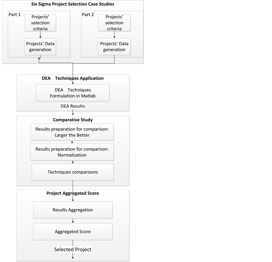
Figure 1. Methodology.
rick scores) are based on the smaller the better. We performed a two-step normalization for the Maverick based scores. First we use Equation (11) to transform the Maverick scores into the larger the better.
 (11)
(11)
However since some of the Maverick scores are greater than 1 and some are smaller than 1,  would have both positive and negative values; we used max-min standardization technique as shown in Equation (12).
 (12)
(12)
The results of all the formulation are then normalized using Equation (13).
 (13)
(13)
A qualitative comparison between the different DEA techniques is performed to explore the diversity in the ranking of projects produced by the different DEA formulation.
Table 5. Summary of the different DEA models used in the study.
3.4. Project Aggregated Score
The normalized scores are summed to obtain a unified score for each project, thus leading to one score to be used for project selection.
4. Results and Discussion
In Subsection 4.1, we present the results of applied the Multi-DEA USF to the data provided by [6] . In Subsections 4.2 - 4.4, we present the results of the extended datasets.
4.1. Applying the Multi-DEA USF and Validation
For the dataset presented by [6] , we initially applied the simple DEA formulation. Out of the twenty projects, only five projects are efficient. Then, we applied all the other DEA formulations to this dataset. Table 6 present the scores of the five efficient projects. The complete list of scores for the twenty projects is shown in Table 14 (Appendix II) which coincides perfectly with the results provided by [6] .
In Table 6, we notice that the Aggressive and Benevolent scores are less than the simple score for each project. This agrees with the logic of the simple CCR formulation where each project maximizes its own score; while, in the Aggressive and Benevolent formulations a secondary goal constrains the problem and prevents the project from achieving better than its simple score.
Also, note that a lower Maverick score means that the project is less of a Maverick which gives the project a higher rank.
It can be noticed that not all the DEA formulations agreed on the selected projects. For the above case all DEA formulations have selected project 7 except for the aggressive technique which selected project 17. Thus
Table 6. Summary of scores for efficient projects Part 1.
for the data provided by [6] only one of the DEA formulations have disagreed with the rest. However, this cannot be generalized to other cases as will be shown in the next subsection.
The normalized scores for each efficient project were calculated and compared using Figure 2. The normalized scores coincides perfectly with the data provided in Table 5. In that, Project 7 seems to outperform the rest of the projects in all formulations except for the aggressive technique.
Figure 3 presents the aggregated score for the efficient projects. Project 7 is identified as the best six sigma project. This figure shows that project 7 outperforms the rest of the projects and has a clear edge for selection.
4.2. Applying the Multi-DEA USF for the Extended Data Sets
We initially applied simple efficiency to select the efficient projects. Then we applied the rest of the DEA formulations. Table 7 and Figure 4 present the scores of the efficient projects. Comparing the efficient projects is more cumbersome in this case because more projects are efficient (14 projects).
The selected project for each DEA formulation is shown in Bold. It’s clear from Table 7 and Figure 4 that the DEA formulations have diverse decisions. Project 7 has been selected by three DEA formulations, project 19 has been selected by three as well, while project 3 is selected by two and project 10 is selected by one DEA formulation. Thus, the selection process was extremely difficult and requires a rigorous method. The reason of this is the high competitively between the projects. The different DEA techniques are showing high variability in terms of the project expected cost, the best project is project 7. While for expected project duration project 12 is the shortest. Level of management commitment project is 8 the best, etc. For this reason, there was high variability in terms of the selected project using different DEA techniques. For example, aggressive formulation choose project 10. The aggressive cross efficiency choose project 19. The benevolent cross efficiency choose project 7 to be the best project. This diverse decision phenomenon places a lot of doubts on how to pick up the winning one. It is also stresses the need for a unified methodology for choosing the finalized winning project. We suggest in this work to use the Multi-DEA-USF for this purpose.
Figure 5 shows the final aggregate score for the different projects. The suggested technique have successfully selected project 17, although project 7 was a close competing peer project. Figure 6 illustrates why this important project should be selected, although it was pick up by only one DEA-formulation (Aggressive) as the winning project. This important project-which might have gone unnoticed through applying only the individual DEA formulations-was always a close competitor in all DEA formulations to the leading projects 7 and 19. It performed better than them in terms of the aggressive scores. The successful selection of project 17-which was shadowed by project 7 and 19 is a major advantage of the suggested technique (multi-DEA-USF) over the individual DEA formulations which allows shadowing of close competitors. The close competitor gives a more stable performance (always performing good enough) in all DEA formulations while the projects picked up by some of the DEA formulations might have worse performance in others (example project 19 in Mav_Bnv).
4.3. Applying the Multi-DEA USF to 2nd Dataset
Following to simple DEA application we applied all DEA formulations devised have been applied. Table 8 and Figure 7 show the performance index for each project with respect to each DEA formulation. The selected project by each formulation is in highlighted in bold font. The selection process is highly diverse and it is extremely difficult to pick up a winning project.
Figure 2. Normalized score for different DEA formulations for efficient projects.

Figure 3. Aggregated scores
Table 7. Summary of scores for efficient projects Part 2 (1st set).
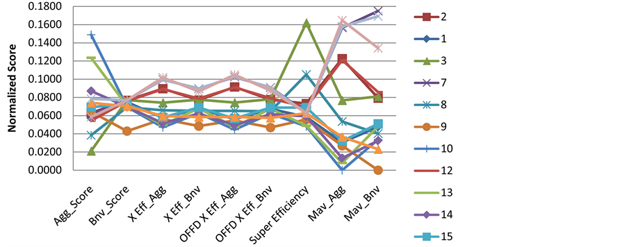
Figure 4. Normalized score for different DEA formulations for efficient projects.
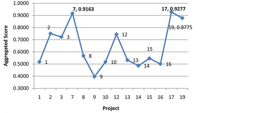
Figure 5. Aggregated score Part 2 (1st set).
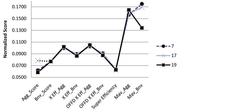
Figure 6. Normalized score for different DEA formulations for competing projects.
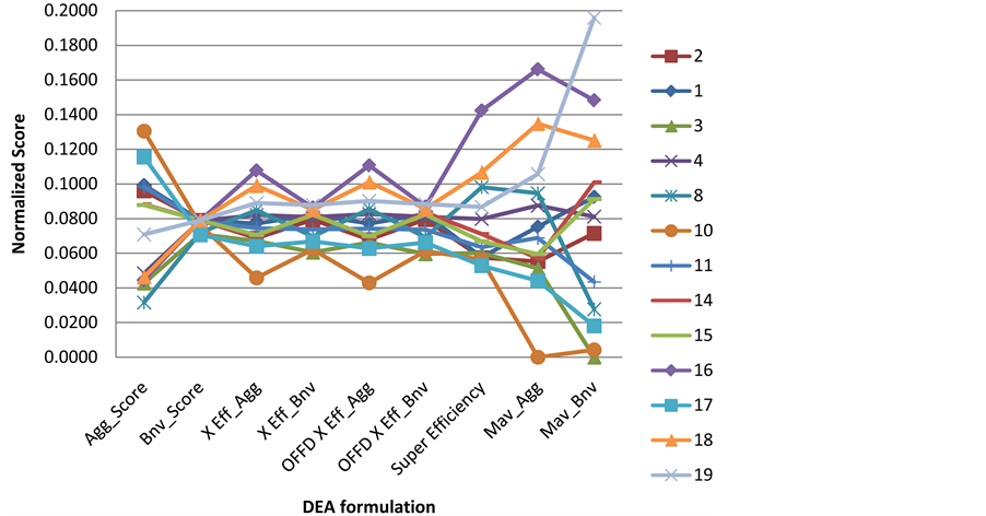
Figure 7. Normalized score for different DEA formulations for efficient projects (2nd set).
Table 8. Summary of scores for efficient projects Part 2 (2nd set).
Figure 7 shows the normalized scores for the different projects, project 16 should be selected while the close competitors are projects 18 and 19.
Figure 8 presents the final aggregate score for the different projects. The suggested technique have successfully selected project 16 although projects 18 and 19 are close competing peer projects.
Figure 9 shows the performance the three competing projects against the different DEA techniques. The figure shows that the project 16 outperforms the other projects in many of the individual DEA techniques. The Multi-DEA-USF was successful in picking up a highly performing project.
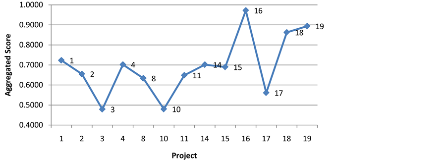
Figure 8. Aggregated score Part 2 (2nd set).
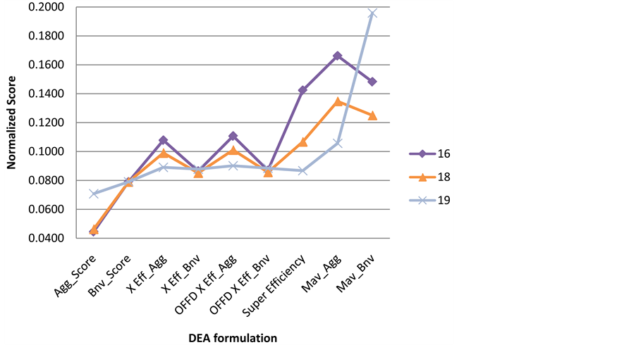
Figure 9. Normalized score for different DEA formulations for competing projects.
4.4. Applying the Multi-DEA USF to the 3rd Set
Table 9 and Figure 10 show the performance index for each project with respect to each DEA formulation. It look like that project 1 is highly competitive as it was picked up by some of the DEA techniques. Project 11 shows also some competitive advantage as it has been picked also by some of the individual DEA formulations.
Figure 11 shows the aggregate result for the different projects using the Multi-DEA-USF. Project 1 is the winning project with no close competitors in terms the aggregate index. The Multi-DEA-USF was successful in selecting a highly competitive project.
5. Conclusions
The Multi-DEA-USF proposed in this work is used to solve the important six sigma project selection problem which is multi criteria-multi objective. DEA has been used to solve this problem. This work initially solves the six sigma project selection problem using the several DEA formulations proposed in the literature, and concludes that different formulation can give different results in terms of the projects selected. To overcome this diverse DEA result problem, this work proposes using simple normalization and simple weighted score summing as a unified approach to select the winning project.
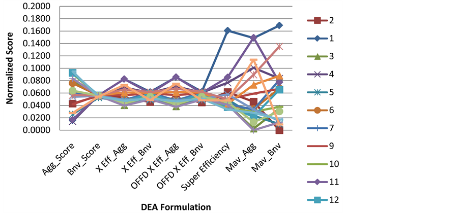
Figure 10. Normalized score for different DEA formulations for efficient projects (3rd set).
Table 9. Summary of scores for efficient projects Part 2 (3rd set).

Figure 11. Aggregated score Part 2 (3rd set).
This framework was applied to several case studies and was always successful in picking up “highly competitive” projects. The Multi-DEA-USF was especially successful in picking up stable and well performing project (performing well in all DEA), even though it might have never been selected by any of the DEA formulations (that were excellent projects “shadowed” by slightly better performing projects) and filtering out projects with selective excellent performance; these were projects performing well in some and less well in other DEA formulations.
References
- Henderson, G.R. (2011) Six Sigma Quality Improvement with Minitab. John Wiley & Sons, Hoboken. http://dx.doi.org/10.1002/9781119975328
- Coronado, R.B. and Antony, J. (2002) Critical Success Factors for the Successful Implementation of Six Sigma Projects in Organisations. The TQM Magazine, 14, 92-99. http://dx.doi.org/10.1108/09544780210416702
- Antony, J., Antony, F.J., Kumar, M. and Rae Cho, B. (2007) Six Sigma in Service Organisations: Benefits, Challenges and Difficulties, Common Myths, Empirical Observations and Success Factors. International Journal of Quality & Reliability Management, 24, 294-311. http://dx.doi.org/10.1108/02656710710730889
- Meredith, J.R. and Mantel Jr., S.J. (2011) Project Management: A Managerial Approach. John Wiley & Sons, Hoboken.
- Saghaei, A. and Didehkhani, H. (2011) Developing an Integrated Model for the Evaluation and Selection of Six Sigma Projects Based on ANFIS and Fuzzy Goal Programming. Expert Systems with Applications, 38, 721-728. http://dx.doi.org/10.1016/j.eswa.2010.07.024
- Dinesh Kumar, U., Saranga, H., Ramírez-Márquez, J.E. and Nowicki, D. (2007) Six Sigma Project Selection Using Data Envelopment Analysis. The TQM Magazine, 19, 419-441. http://dx.doi.org/10.1108/09544780710817856
- Zimmerman, J. and Weiss, J. (2005) Six Sigma’s Seven Deadly Sins. Quality, 44, 62-66.
- Deshmukh, S. and Lakhe, R. (2009) Development and Validation of an Instrument for Six Sigma Implementation in Small and Medium Sized Enterprises. 2nd International Conference on Emerging Trends in Engineering and Technology (ICETET).
- Kazemi, S.M., et al. (2012) Six Sigma Project Selections by Using a Fuzzy Multi Criteria Decision Making Approach: A Case Study in Poly Acryl Corp. CIE42 Proceedings, CIE and SAIIE, 306-1-306-9.
- Wyman, O. (2007) Keystone of Lean Six Sigma: Strong Middle Management. New York.
- Antony, J. and Banuelas, R. (2002) Key Ingredients for the Effective Implementation of Six Sigma Program. Measuring Business Excellence, 6, 20-27. http://dx.doi.org/10.1108/13683040210451679
- Ray, S. and Das, P. (2010) Six Sigma Project Selection Methodology. International Journal of Lean Six Sigma, 1, 293- 309. http://dx.doi.org/10.1108/20401461011096078
- George, M.O. (2010) The Lean Six Sigma Guide to Doing More with Less: Cut Costs, Reduce Waste, and Lower Your Overhead. John Wiley & Sons, Hoboken.
- Larson, A. (2003) Demystifying Six Sigma: A Company-Wide Approach to Continuous Improvement. AMACOM, New York.
- Thomas, P. (2003) The Six Sigma Project Planner. McGraw, New York.
- Pyzdek, T. and Keller, P.A. (2010) The Six Sigma Handbook: A Complete Guide for Green Belts, Black Belts, and Managers at All Levels. 3rd Edition, McGraw-Hill, New York.
- Banuelas, R. and Antony, J. (2007) Application of Stochastic Analytic Hierarchy Process within a Domestic Appliance Manufacturer. Journal of the Operational Research Society, 58, 29-38. http://dx.doi.org/10.1057/palgrave.jors.2602060
- Su, C.T. and Chou, C.J. (2008) A Systematic Methodology for the Creation of Six Sigma Projects: A Case Study of Semiconductor Foundry. Expert Systems with Applications, 34, 2693-2703. http://dx.doi.org/10.1016/j.eswa.2007.05.014
- Kahraman, C. and Büyüközkan, G. (2008) A Combined Fuzzy AHP and Fuzzy Goal Programming Approach for Effective Six-Sigma Project Selection. Multiple-Valued Logic and Soft Computing, 14, 599-615.
- Banuelas, R. and Antony, J. (2003) Going from Six Sigma to Design for Six Sigma: An Exploratory Study Using Analytic Hierarchy Process. The TQM Magazine, 15, 334-344. http://dx.doi.org/10.1108/09544780310487730
- Kelly, W.M. (2002) Three Steps to Project Selection. Six Sigma Forum Magazine, 2, 29-32.
- Adams, C., Gupta, P. and Wilson, C. (2011) Six Sigma Deployment. Routledge, London.
- Pyzdek, T. (2000) Selecting Six Sigma Projects. http://www.qualitydigest.com/sept00/html/sixsigma.html
- Pande, P.S. and Neuman, R.P. (2000) The Six Sigma Way: How GE, Motorola, and Other Top Companies Are Honing Their Performance. 1st Edition, McGraw-Hill, New York.
- Kumar, M., Antony, J. and Cho, B.R. (2009) Project Selection and Its Impact on the Successful Deployment of Six Sigma. Business Process Management Journal, 15, 669-686. http://dx.doi.org/10.1108/14637150910987900
- Charnes, A., Cooper, W.W. and Rhodes, E. (1978) Measuring the Efficiency of Decision Making Units. European Journal of Operational Research, 2, 429-444. http://dx.doi.org/10.1016/0377-2217(78)90138-8
- Cooper, W.W., Seiford, L.M. and Zhu, J. (2011) Handbook on Data Envelopment Analysis. Springer, Berlin.
- Lim, S. (2010) A Formulation of Cross-Efficiency in DEA and Its Applications. 40th International Conference on Computers and Industrial Engineering (CIE).
- Despotis, D.K. (2002) Improving the Discriminating Power of DEA: Focus on Globally Efficient Units. The Journal of the Operational Research Society, 53, 314-323. http://dx.doi.org/10.1057/palgrave.jors.2601253
- Charnes, A., Cooper, W.W., Lewin, A.Y. and Seiford, L.M. (1994) Data Envelopment Analysis: Theory, Methodology and Applications. Springer, Berlin.
- Liang, L., Wu, J., Cook, W.D. and Zhu, J. (2008) Alternative Secondary Goals in DEA Cross-Efficiency Evaluation. International Journal of Production Economics, 113, 1025-1030. http://dx.doi.org/10.1016/j.ijpe.2007.12.006
- Anderson, T.R., Hollingsworth, K. and Inman, L. (2002) The Fixed Weighting Nature of a Cross-Evaluation Model. Journal of Productivity Analysis, 17, 249-255. http://dx.doi.org/10.1023/A:1015012121760
- Doyle, J. and Green, R. (1994) Efficiency and Cross-Efficiency in DEA: Derivations, Meanings and Uses. The Journal of the Operational Research Society, 45, 567-578. http://dx.doi.org/10.1057/jors.1994.84
- Charnes, A., Haag, S., Jaska, P. and Semple, J. (1992) Sensitivity of Efficiency Classifications in the Additive Model of Data Envelopment Analysis. International Journal of Systems Science, 23, 789-798. http://dx.doi.org/10.1080/00207729208949248
- Andersen, P. and Petersen, N.C. (1993) A Procedure for Ranking Efficient Units in Data Envelopment Analysis. Management Science, 39, 1261-1264. http://dx.doi.org/10.1287/mnsc.39.10.1261
- Zhu, J. (2003) Quantitative Models for Performance Evaluation and Benchmarking: Data Envelopment Analysis with Spreadsheets and DEA Excel Solver. Vol. 51, Springer, Berlin.
Appendix I: Data for Projects’ Input/Output (Tables 10-13)
Table 10. The input and output data for the six sigma projects [6] .
Table 11. The input and output data for the six sigma projects Part 2 (1st set).
Table 12. The input and output data for the six sigma projects Part 2 (2nd set).
Table 13. The input and output data for the six sigma projects Part 2 (3rd set).
Appendix II: Summary of Projects’ Scores (Tables 14-17)
Table 14. Summary of project scores Part 1.
Table 15. Summary of project scores Part 2 (1st set).
Table 16. Summary of project scores Part 2 (2nd set).
Table 17. Summary of project scores Part 2 (3rd set).