American Journal of Operations Research
Vol.3 No.6(2013), Article ID:38455,11 pages DOI:10.4236/ajor.2013.36045
A Genetic Algorithm for Multiple Inspections with Multiple Objectives
School of Business, Wake Forest University, Winston-Salem, USA
Email: mcmullpr@wfu.edu
Copyright © 2013 Patrick R. McMullen. This is an open access article distributed under the Creative Commons Attribution License, which permits unrestricted use, distribution, and reproduction in any medium, provided the original work is properly cited.
Received August 28, 2013; revised September 28, 2013; accepted October 5, 2013
Keywords: Component; Formatting; Style; Styling; Insert
ABSTRACT
This research presents a genetic algorithm to address the problem where multiple inspections are done to test conformity of multiple product characteristics. The genetic algorithm is employed to find an inspection plan where the multiple inspections are carried out, motivated to optimize two objectives: minimization of the total cost associated with the inspection; and maximization of probability of accepting conforming units. The genetic algorithm includes a constraint to induce variety into the characteristics being tested, so that the inspections are not dominated by “specialized” product characteristics. The resulting solutions are compared to optimal solutions, and it is determined that formidable solutions are found via the Genetic Algorithm approach.
1. Introduction
An important aspect of the quality assurance function in manufacturing is deciding how to implement inspection stations for multiple-stage manufacturing. The general consequence of sub-optimal implementation of multiple inspection stations is essentially twofold: first, 100% inspection and/or too many inspection stations become expensive; and second, too few inspection stations will likely result in non-conforming units being sent to the customer, resulting very unpleasant circumstances for all stakeholders involved [1].
Another force complicating this issue is the situation where inspection errors are possible [2-7]. In this context, there are essentially two types of inspection errors that are possible: the first type is where a conforming unit is incorrectly classified as non-conforming; the second type is where a non-conforming unit is incorrectly classified as conforming. The former is referred to as a Type I error, while the latter is referred to as a Type II error. Both of these errors are costly, but it is typical for a Type II error to have a high per unit cost as compared to a Type I error, because of the residual problems of shipping a non-conforming unit to the customer.
Yet another force complicating this issue is the situation where the items requiring inspection have many different attributes or characteristics that require inspection [8-12]. An electronic assembly is a good example of this —many different features of an electronic assembly may require inspection. It is also possible that some of these specific features may require inspection multiple times, due to the subsequent value adding activities that occur during the assembly and/or manufacturing. For example, the power supply of a desktop computer may require inspection or conformance testing before and after the power supply is connected to the system board.
Additionally, some attributes of a manufactured or assembled item may not require testing at all. An example of this might be an electrical connection in an assembly. The testing of this characteristic may be considered unnecessary due to the consistent reliability of the connection. In circumstances such as this, it might be appropriate to direct inspection resources to more critical attributes of the manufactured item.
It is also important to note that for each type of attribute requiring inspection, there may be differing inspection costs, and differing probabilities of conformities and differing probabilities of acceptance. The consequence of this is that determining the cost of an inspection plan, along with determining the probability of conforming units being accepted through all stages of inspection via the inspection plan is far from trivial.
In the face of the complicating forces detailed above, it is desired to design an inspection plan in a minimal-cost fashion. This cost is an aggregation of inspection costs, total cost of rejecting conforming units and the total cost of accepting non-conforming units. It is desired to find an inspection plan such that the “best” overall aggregation of these entities is found. At the same time, however, constraints need to apply such that “cheaper” attribute inspections do not dominate the inspection plan. In other words, it is imperative to mandate that the inspection plan is not dominated by attribute inspections that will “drive down” the total cost. A minimum number of unique attribute inspections are needed specified to prevent dominance.
Additionally, cost is not the only element that could be considered when seeking to find an optimal inspection plan [13]. While cost is an important metric of an inspection plan (perhaps the most important), there are other entities that could be considered. One important entity of an inspection plan, aside from cost, is maximizing the probability of conforming items that “survive” the inspection process. That is, maximizing the number of units that are accepted after the final inspection station. In layman’s terms, it is desired to have as many finished units as possible sent to the customer. While the cost of rejecting conforming units is included in the cost function, it is still desired to maximize the number of conforming units that “survive” the inspection process, so as to maximize long-term revenue.
As was the case for minimizing cost, it is also important to constrain the number of unique items that comprise the inspection plan when seeking to maximize the number of units that “survive” inspection through the final inspection station. This is necessary so as to avoid specific attributes being repeatedly inspected that result in high probabilities of “surviving” inspection through the last station.
As such, the present research effort simultaneously considers two objectives for optimization: minimization of cost associated with the inspection plan, and maximization of the expected value of conforming units being accepted. While these multiple objectives are pursued, there does exist a constraint imposing a minimal number of unique characteristics present in the inspection plan, so as to avoid certain characteristics from dominating the resultant inspection plan. This is considered a unique feature of this research effort—the authors are not aware of other efforts that give consideration to this issue.
Finding an optimal solution to problems of this type is quite difficult due to the combinatorial nature of the problem. If there are m unique product attributes that could be tested, and n tests that are required, there can be, in the absence of constraints, as many as mn possible inspection plans. Because of this combinatorial difficulty, larger problem instances cannot be solved to guaranteeoptimality. Instead, some sort of heuristic is needed to obtain a solution to large problems. For this research effort, a Genetic Algorithm is employed to find desirable inspection plans, in terms of the aforementioned objectives, for several test problems. A genetic algorithm was chosen as the heuristic because of this ability to create and manipulate sequences—for all intents and purposes, and the details of an inspection plan can easily be thought of as a “sequence”.
The following sections will detail the computational aspects of this problem, provide a Genetic Algorithm methodology to solve the problem, employ the Genetic Algorithm on a set of test problems, compare the Genetic Algorithm results to optimality, and offer concluding comments and a general perspective on the state of this problem.
2. The Multiple-Stage Sequencing Problem
Prior to describing the multiple-stage sequencing problem, a few relevant terms are defined in Table 1. Given these terms, the multiple-stage inspection model is detailed in Figure 1.
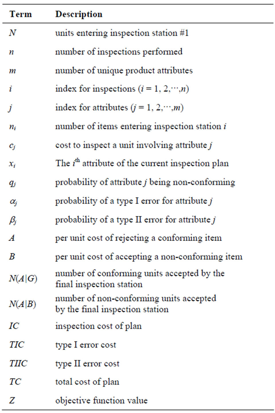
Table 1. Terms used to describe multiple-stage sequencing problem.
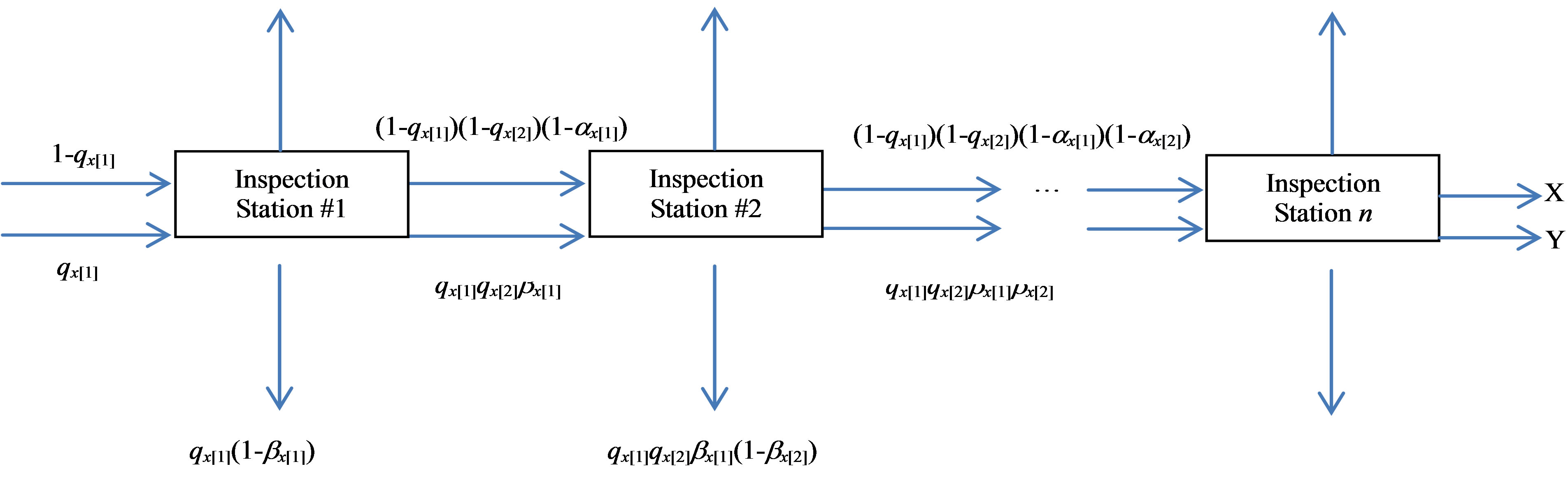
Figure 1. Layout of inspection stages.
The upward pointing arrows denote conforming items that are rejected (Type I errors). The downward pointing arrows denote non-conforming items that are rejected. The entity denoted by “X” represents the proportion of conforming units that are accepted. When multiplied by the number of units entering the first inspection station, we are provided with the expected value of conforming units that are accepted through the nth inspection station—an objective function value of interest. Mathematically, this is as follows:
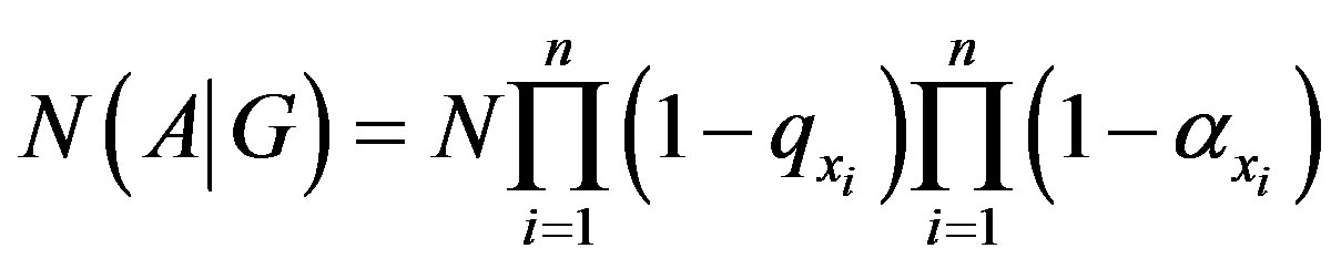 (1)
(1)
The entity denoted by “Y” represents the proportion of non-conforming units that are accepted (Type II errors). When multiplied by N, the number of units entering the first inspection station, it represents the expected value of non-conforming units accepted at the nth inspection station. Mathematically, this is as follows:
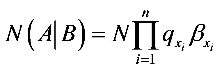 (2)
(2)
The other objective function value of interest is the cost associated with the inspection plan. The cost is comprised of three components: the cost of inspecting items at each of the n inspection stations; the number of conforming units rejected at the n inspection stations (treated here as an opportunity loss); and the number of nonconforming units that are accepted at the nth inspection station and sent to the customer.
The cost of inspecting items through all n inspection stations is the total number of units inspected through all stations, multiplied by the inspection cost at that particular station. Mathematically, this is as follows:
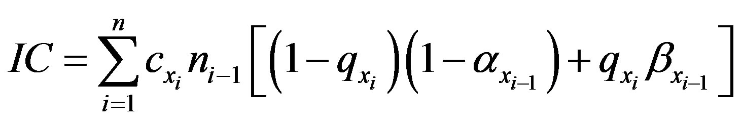 (3)
(3)
In this formula, n0 is initialized to N, while α0 is initialized to 0, and β0 is initialized to 1. In essence, the inspection cost at station i is a function of the number of units surviving inspection through the prior (i − 1) inspection station. As a matter of full disclosure, ni is as follows:
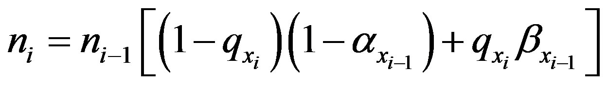 (4)
(4)
The total cost of rejecting units that should be accepted is as follows:
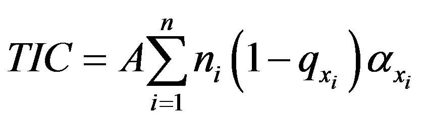 (5)
(5)
The cost of accepting non-conforming units at the nth inspection station is as follows, which is an expansion of Equation (2):
 (6)
(6)
The total cost, then, of the inspection plan is the sum of the inspection cost, the Type I error cost, and the Type II error cost. Mathematically, this is as follows:
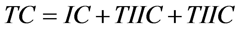 (7)
(7)
In terms of the terms defined in Table 1, the total cost is as follows:
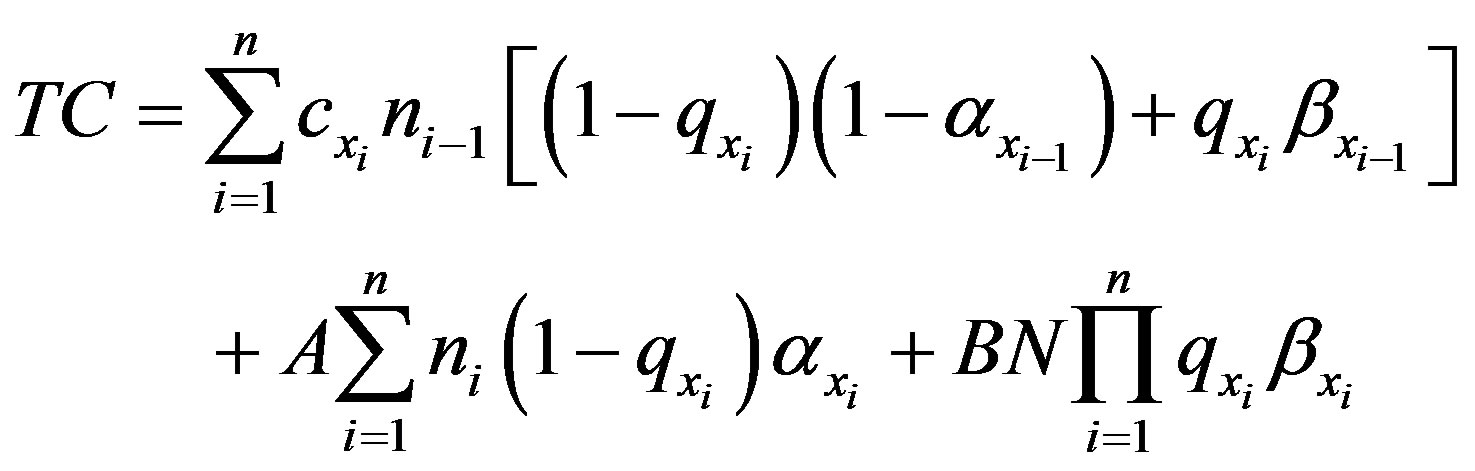 (8)
(8)
As stated earlier, the intent for this research is to optimize two objectives: maximization of N(A|G) and minimization of TC. To do this, a ratio involving the two objectives can be constructed:
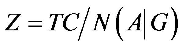 (9)
(9)
Given that it is intended to minimize TC and maximize N(A|G), it is intended to minimize the Z.
3. Finding a Desirable Inspection Plan
As stated earlier, there are m item characteristics that can be tested and n tests to be performed. This means that there can be many possible inspection plans. Specifically, in the absence of constraints regarding unique attributes to be inspected, there can be as many as mn unique inspection plans. Again, this upper bound assumes no limitations on the number of times a specific attribute can be inspected. In the presence of constraints dictating a limitation on the number of times a unique attribute can be inspected, there can be as few as m!/(m − n)! possible inspection plans. This lower bound assumes the extreme case where each attribute can be inspected one time at most (U = n).
Even at the lower bound, the number of unique possible inspection plans is combinatorial in nature, implying that a guaranteed optimal solution is difficult to obtain. Integer and/or nonlinear programming approaches can be used to address problems of this variety, but they also have complicating characteristics [6,7,11]. The same can be said for dynamic programming approaches [14,15]. Because of this, search heuristics become a necessary course of action to find inspection plans desirable with respect to the objective functions.
Genetic Algorithms are well-suited for a problem of this type. Genetic Algorithms have the ability to construct and manipulate sequences motivated by an objective function. In this context, an inspection plan can be thought of as a sequence—a list of length n, where each of the n elements can take on one of m possible values. Through the Genetic Algorithm trademarks of selection, crossover and mutation, a population of inspection plans can be obtained which will, hopefully, result in inspection plans with desirable objective function values. The interested reader is referred to the work of Goldberg [16] and that of Michalewicz and Fogel [17] for a detailed description of the inner-workings of Genetic Algorithms, along with many informative examples.
Prior to describing the specific Genetic Algorithm used here, some specific definitions are stated in Table 2.
3.1. Genetic Algorithm Process
The following sub-sections will describe the details of
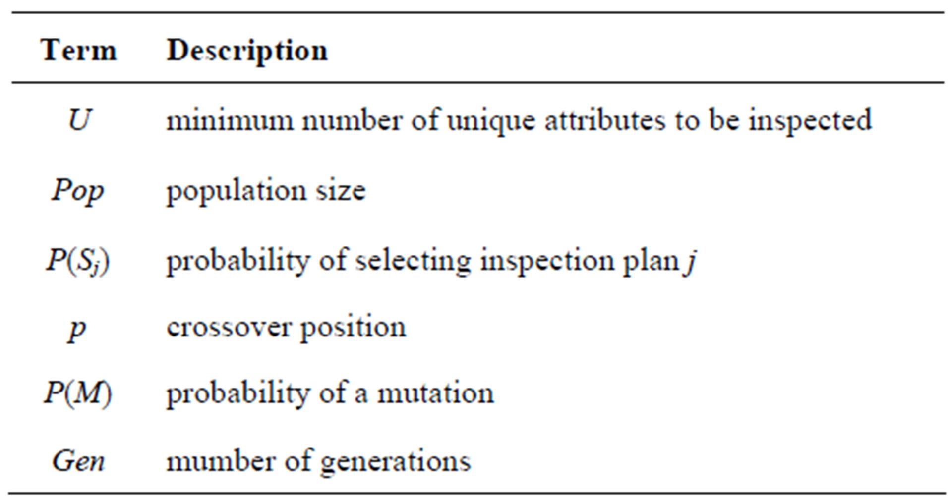
Table 2. Terms used to describe genetic algorithm.
the Genetic Algorithm used to find inspection plans motivated to optimize the objectives of minimum cost and maximization of N(A|G).
3.1.1. Initialization
A population of feasible solutions (inspection plans) is randomly generated. Specifically, attributes to be inspected are randomly selected in the [1, m] interval for all n inspections needed. This random generation of a feasible solution is repeated until the number of unique attributes to be inspected is at least U. The random generation of feasible solutions is repeated in this fashion Pop times.
3.1.2. Selection
For each of the Pop solutions, the objective function value is determined via Equation (9). All objective function values (Z) in Pop are given the index j , the maximum value is referred to as max(Z), and is used to determine the probability of selecting inspection plan j, P(Sj), via the following:
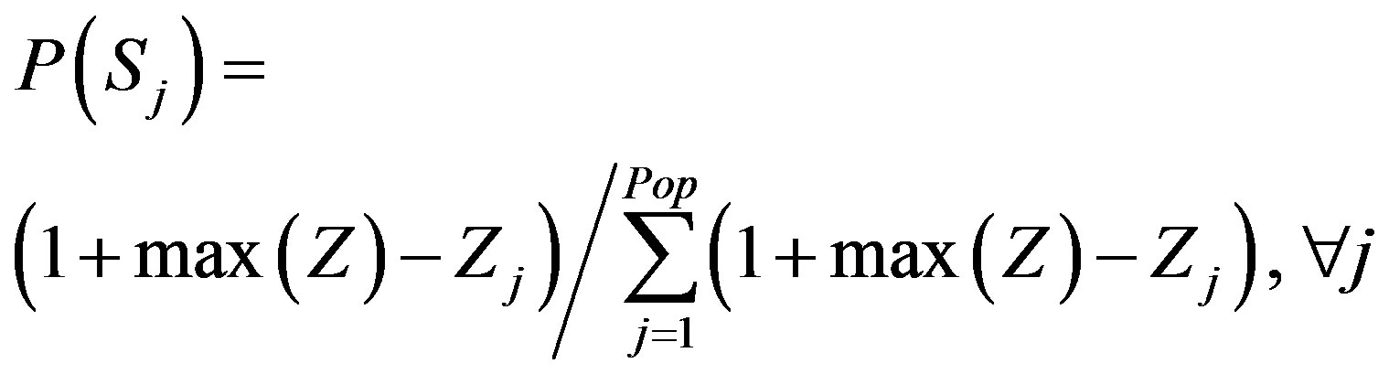 (10)
(10)
This relationship is constructed such that the solutions with the lowest objective function value (value of Z), have the highest probability of being selected, so that its characteristics can be “passed on” to the next generation. Monte Carlo simulation is used to select all Pop members of the new population.
3.1.3. Crossover
The members of the population are put into Pop/2 couples. Members 1 and 2 comprise the first couple, members 3 and 4 comprise the second couple, and so on. For each couple, crossover is performed, by randomly selecting a crossover point, p, on the [2, m − 1] interval. At that point, the attributes to be inspected from the pth position to the mth position are swapped for each couple. To illustrate this, an example is provided, where m is 8, and n is 8. Before crossover, the two inspection plans are coupled, where p = 3.
ABCDEFGH BBAGCHDE The underlined section denotes the attributes to be inspected marked for crossover. After crossover, the following inspection plans result:
ABAGCHDE BBCDEFGH For purposes of full disclosure, the first inspection plan prior to crossover shows eight unique items for inspection, while the second shows seven unique attributes to be inspected. After crossover, the first inspection plan shows seven unique attributes to be inspected, while the second also shows seven. This particular example does not apply any constraint regarding a minimum number of unique attributes to be inspected.
For each couple, crossover is repeated until the number of unique attributes to be inspected for each inspection plan is at least U.
3.1.4. Mutation
After crossover, each inspection plan is considered for mutation. Mutation for each inspection plan will occur with a probability of P(M). In the event that an inspection plan will be mutated, an attribute to be inspected is randomly selected, with all attributes of the inspection plan being equally likely for selection. This selected attribute will be modified to a different attribute, and this different attribute is selected randomly. For example, consider the inspection plan selected for mutation, where the fourthpositioned attribute is targeted for mutation:
ABAGCHDE After mutation, the following inspection plan is possible, where attribute “G” was randomly changed to “C.”
ABACCHDE As was the case with crossover, mutation will occur to a selected inspection plan until the number of unique items in the inspection plan is at least U.
3.1.5. Iteration and Completion
A single iteration has been complete—a new generation has been selected, crossed-over and mutated. The solutions comprising this new generation have their objective function values re-calculated. It is determined whether or not the new generation contains a solution having the best objective function value (that is, a solution with the lowest value of Z).
This process is repeated Gen times, and at the end of Gen iterations, the “best” solution is returned.
4. Experimentation
4.1. Test Problems
To determine whether or not the Genetic Algorithm approach to this problem is effective, the approach is used on several test problems, solutions are obtained, and these solutions are compared to optimal solutions, where the optimal solutions were obtained via complete enumeration. The test problems come from four data sets, which have differing costs and probabilistic parameters. Their values are detailed in Tables 3-6 below.
Several test problems are derived from each of these four input data sets, each exploiting feasible combinations of number of inspections to perform (n) for each inspection plan, along with at least three unique items to
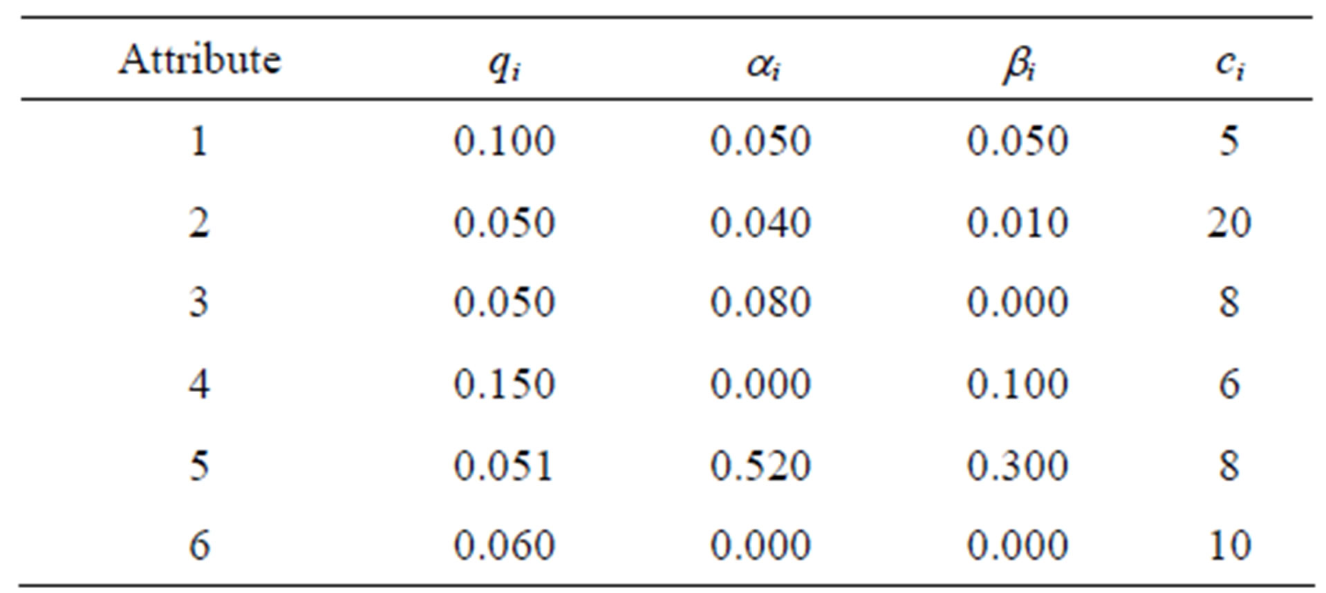
Table 3. Input set 1.
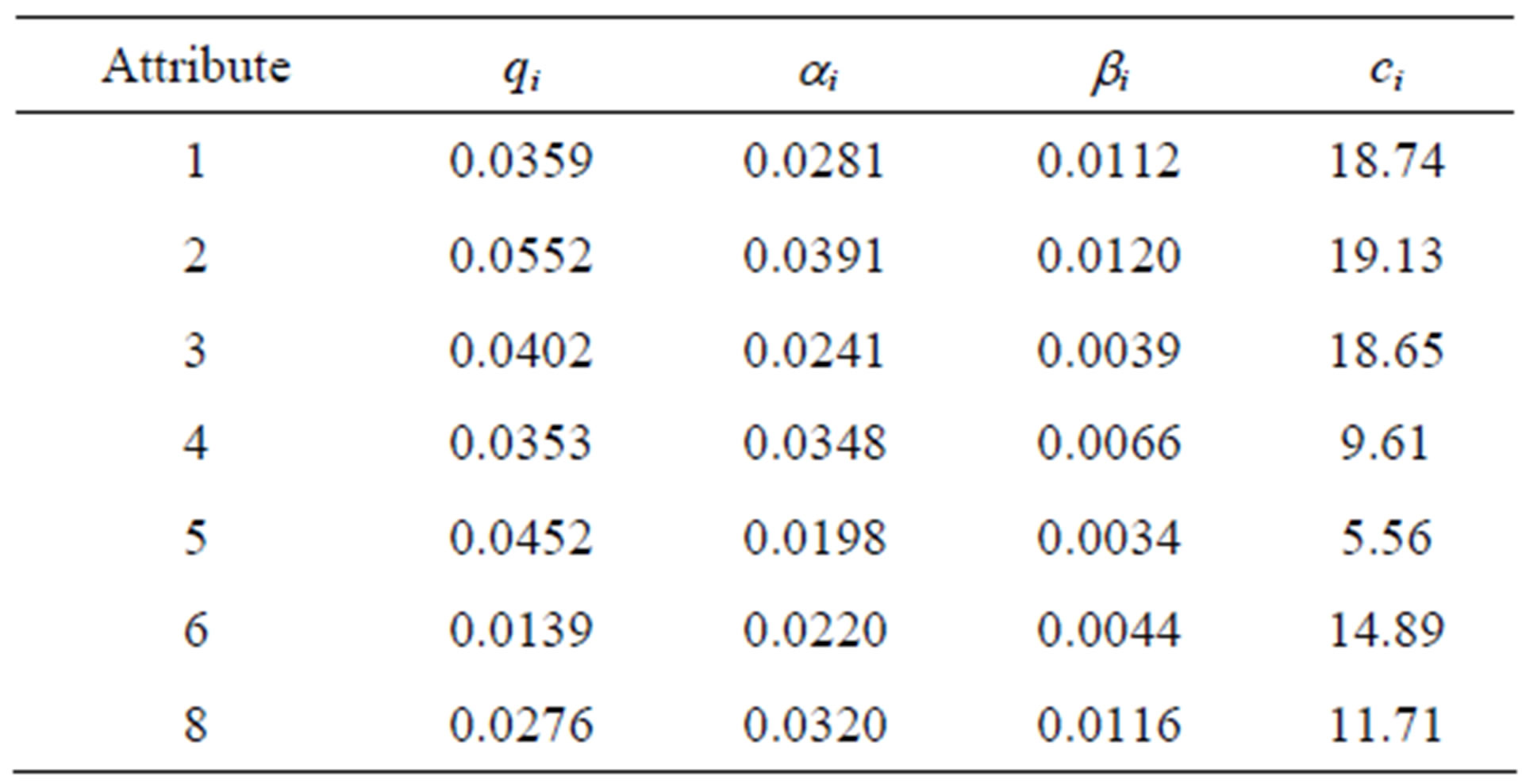
Table 4. Input set 2.
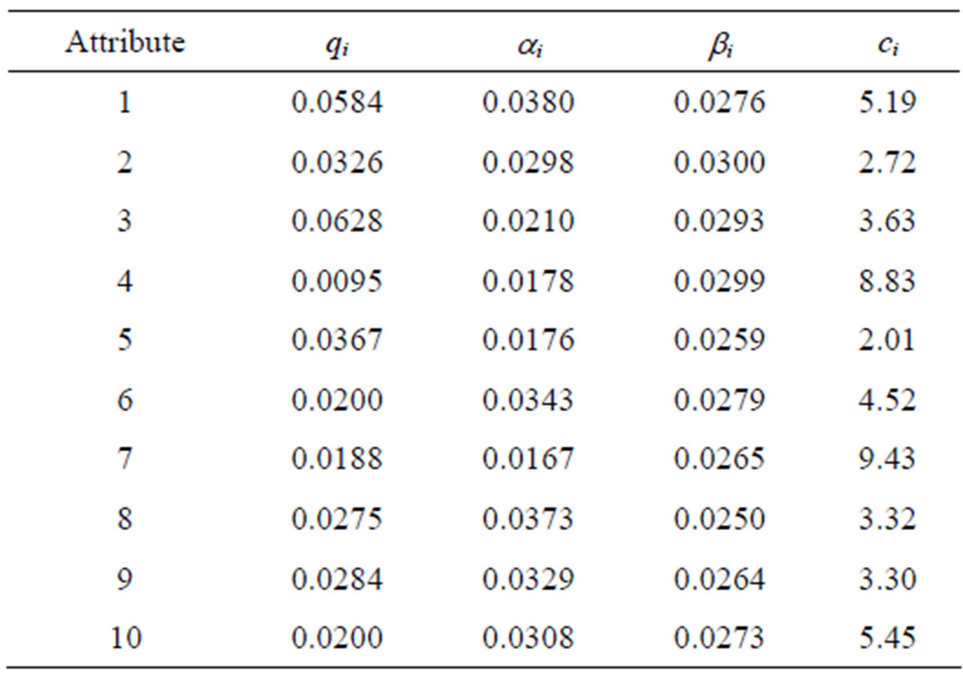
Table 5. Input set 3.
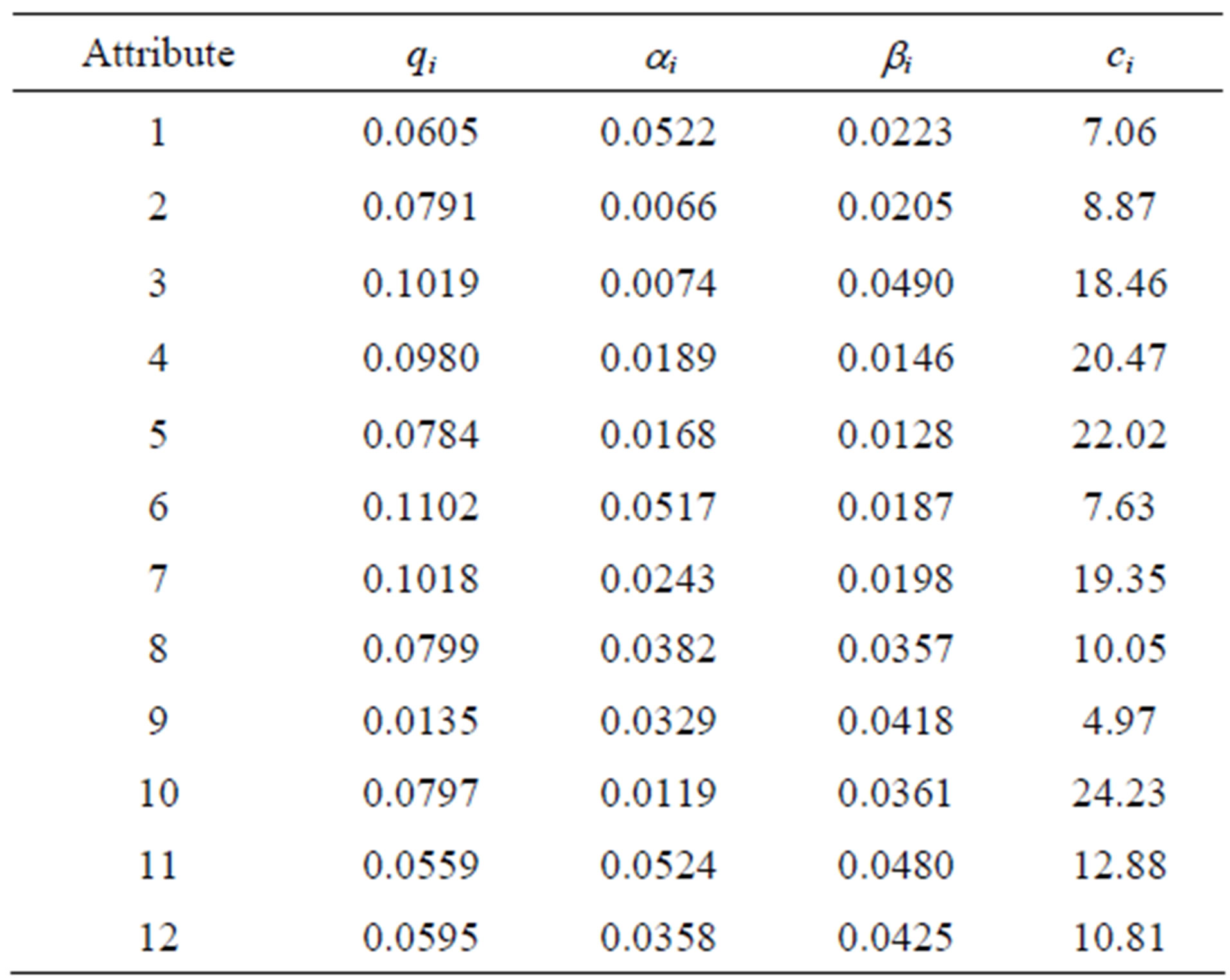
Table 6. Input set 4.
be inspected for each inspection plan (U ³ 3).
Each feasible combination of number of inspection attributes (m) and number of inspections to perform (n) for at least three unique attributes to inspect yields ninety test problems.
4.2. Comparison to Optimal
Each of these ninety problems is solved to optimality via complete enumeration of all feasible inspection plans. For each problem, three performance measures are captured: the minimum cost (TC); the maximum number of conforming units accepted at the final inspection station (N(A|G)); and the minimum objective function value (Z). For each problem, these three optimal values are compared to the values obtained via the Genetic Algorithm.
Formal hypothesis testing is performed to see if there are any significant differences between the results obtained via enumeration and the results obtained via the Genetic Algorithm.
Specifically, the relative inferiority of the objective function value (Z) of the Genetic Algorithm to the optimal value is obtained via the following:
 (11)
(11)
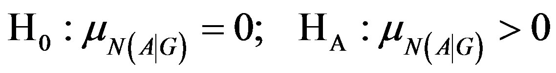
The Relative Inferiority value is determined for all ninety test problems, and the mean is used as the sample mean for the following hypotheses:
 (H1)
(H1)
For total cost associated with the inspection plan, the same logic applies for Relative Inferiority:
 (12)
(12)
Hypotheses are constructed in a similar fashion as above
 (H2)
(H2)
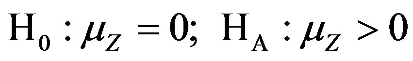
Finally, for the number of conforming units accepted through the nth inspection station, we have the following Relative Inferiority measure:
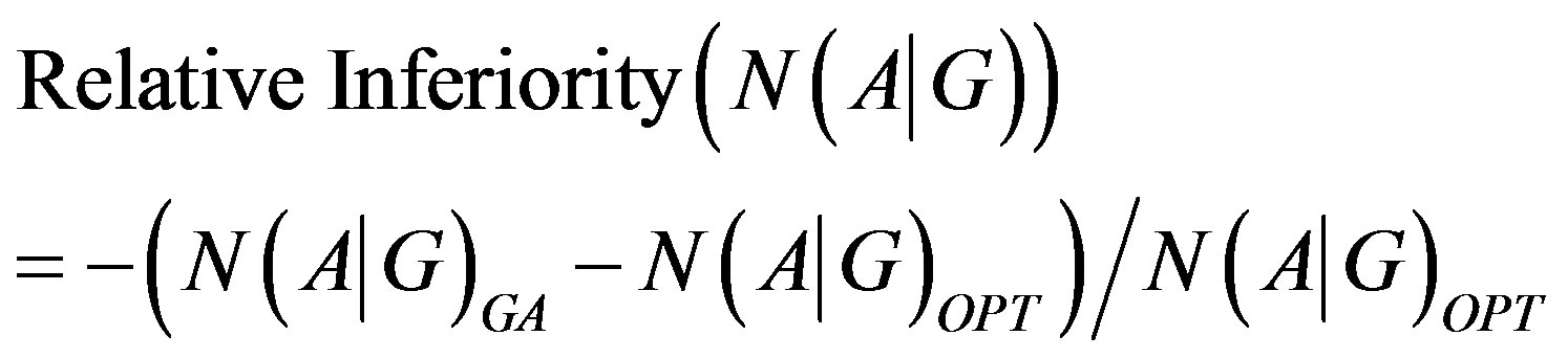 (13)
(13)
The relevant hypotheses for this question are constructed as follows:
 (H3)
(H3)
4.3. Computational Experience
Both the Genetic Algorithm approach described above and the enumeration approach were programmed using the C++ programming language, compiled via the Cygwin compiler, and run on Dual Intel Pentium E2180 processors with a clock speed of 2.00 GHz. The operating system was Windows Vista.
Computational efficiency was always a priority. The Genetic Algorithm Parameters were as follows for the differing problem sets as shown in Table 7.
5. Experimental Results
5.1. Presentation of Results
Tables 8-11 show the results from the ninety test problems obtained via both enumeration and by the Genetic Algorithm. The results are presented by each combination of attributes to inspect (m) and the minimum number of unique attributes to inspect (U) for each input data set. Each m and U cell combination in the table shows the results obtained via enumeration on the first line, with the results obtained via the Genetic Algorithm on the second line. The first entry on each line is the minimum total cost (TC) found for all feasible inspection plans, the second entry on each line is the maximum N(A|G) value found for each feasible inspection plan, while the third entry on each line is the minimum ratio (Z) found for each feasible inspection plan. The fourth entry on the first line, in boldface, is the number of feasible inspection plans—this value is obtained via complete enumeration.
To better understand these tables, an example is provided. Specifically, Table 9(a), for the cell detailing at least six unique items (U ³ 6) and eight inspections to be performed (n = 8) for eight possible attributes (m = 8), the details are shown below in Table 12 in a more decompressed fashion.
For this particular problem, there are 6,531,840 feasible solutions. Comparing the results obtained via Enumeration with the results obtained via the Genetic
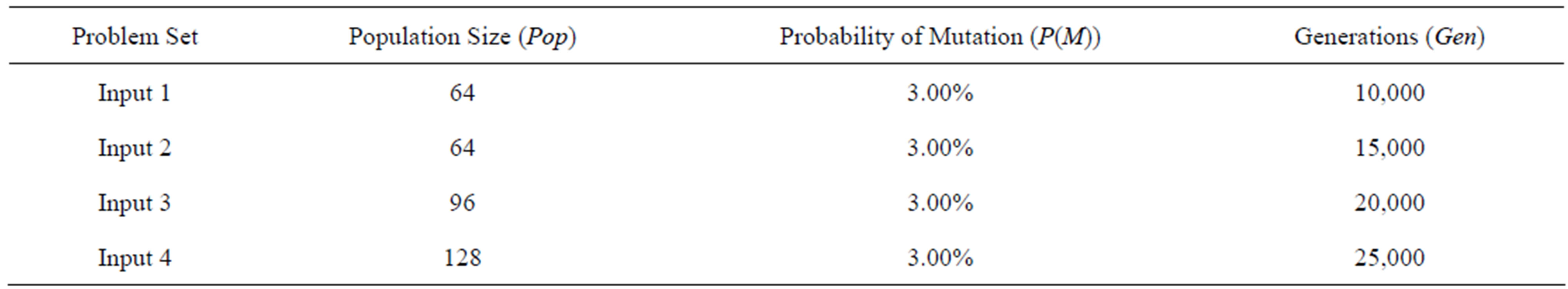
Table 7. Genetic algorithm parameters.
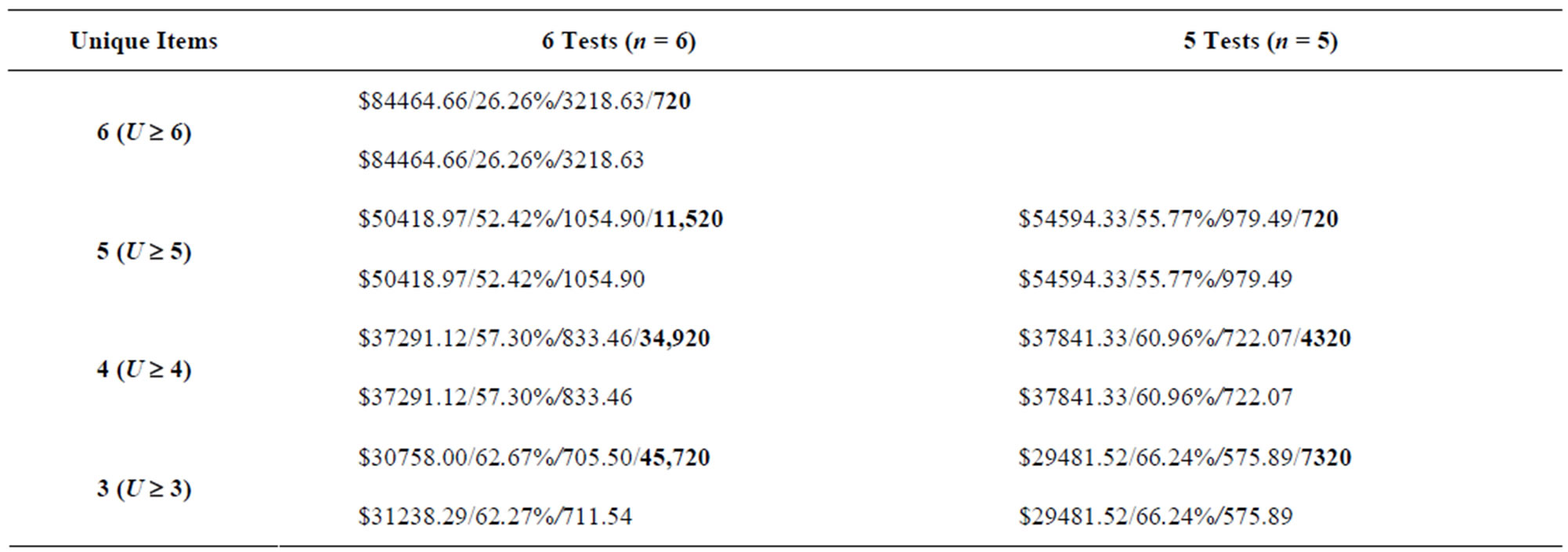
Table 8. Results from input1 data set (m = 6).
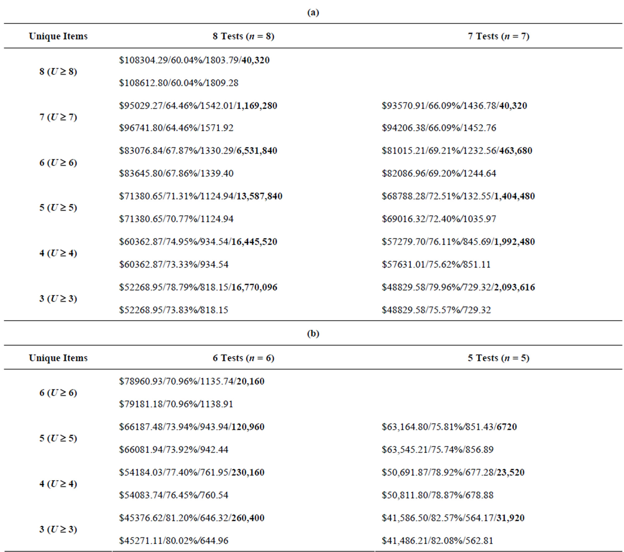
Table 9. (a) Results from input2 data set, 8 tests and 7 tests (m = 8); (b) Results from input2 data set, 6 tests and 5 tests (m = 8).
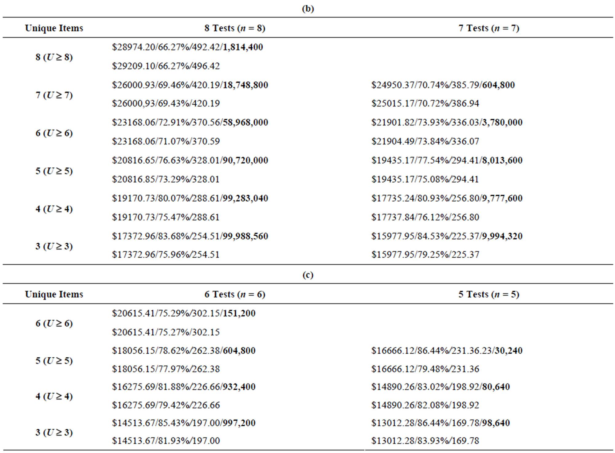
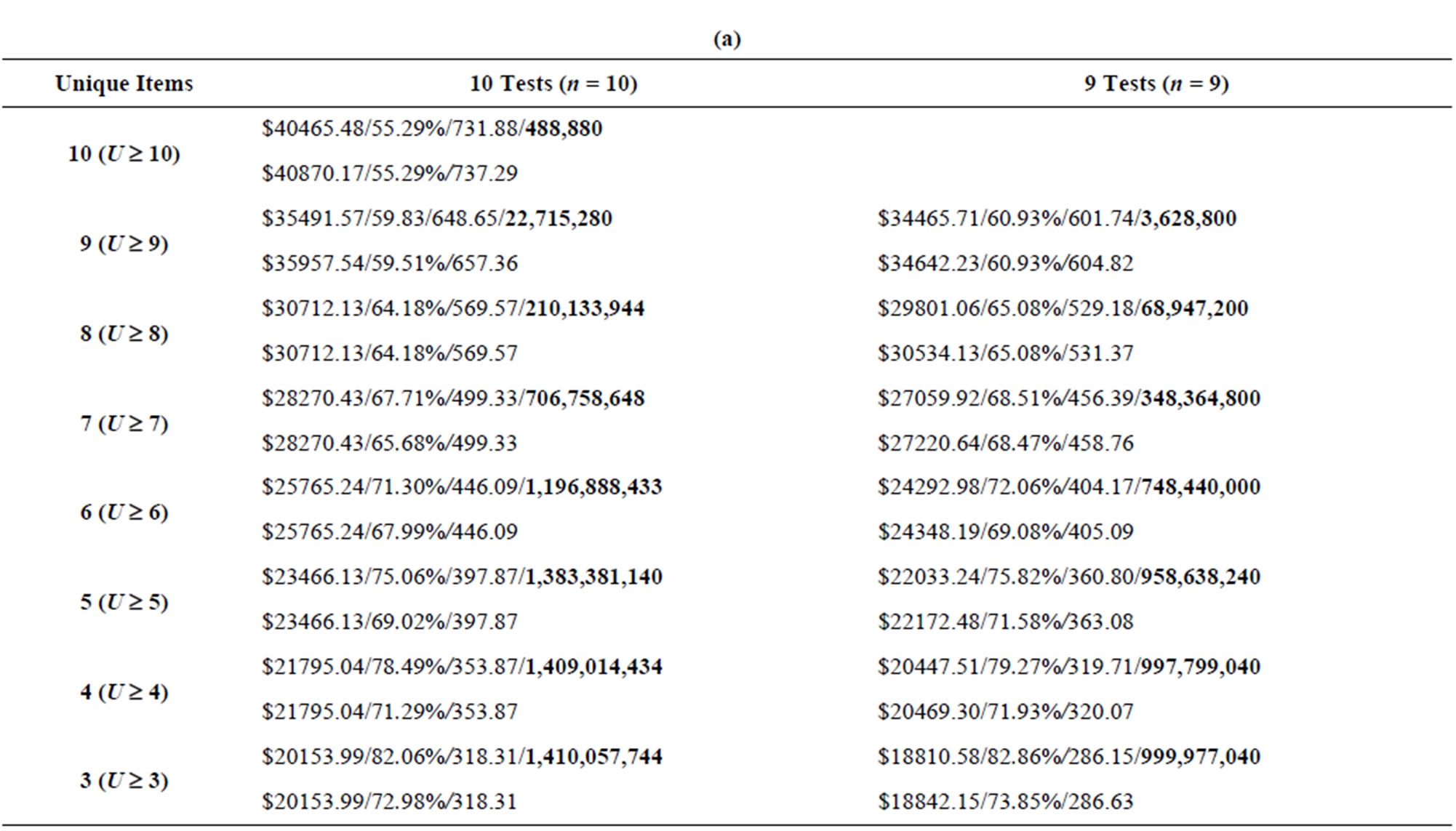
Table 10. (a) Results from input3 data set, 10 tests and 9 tests (m = 10); (b) Results from input3 data set, 8 tests and 7 tests (m = 10); (c) Results from input3 data set, 6 tests and 5 tests (m = 10).
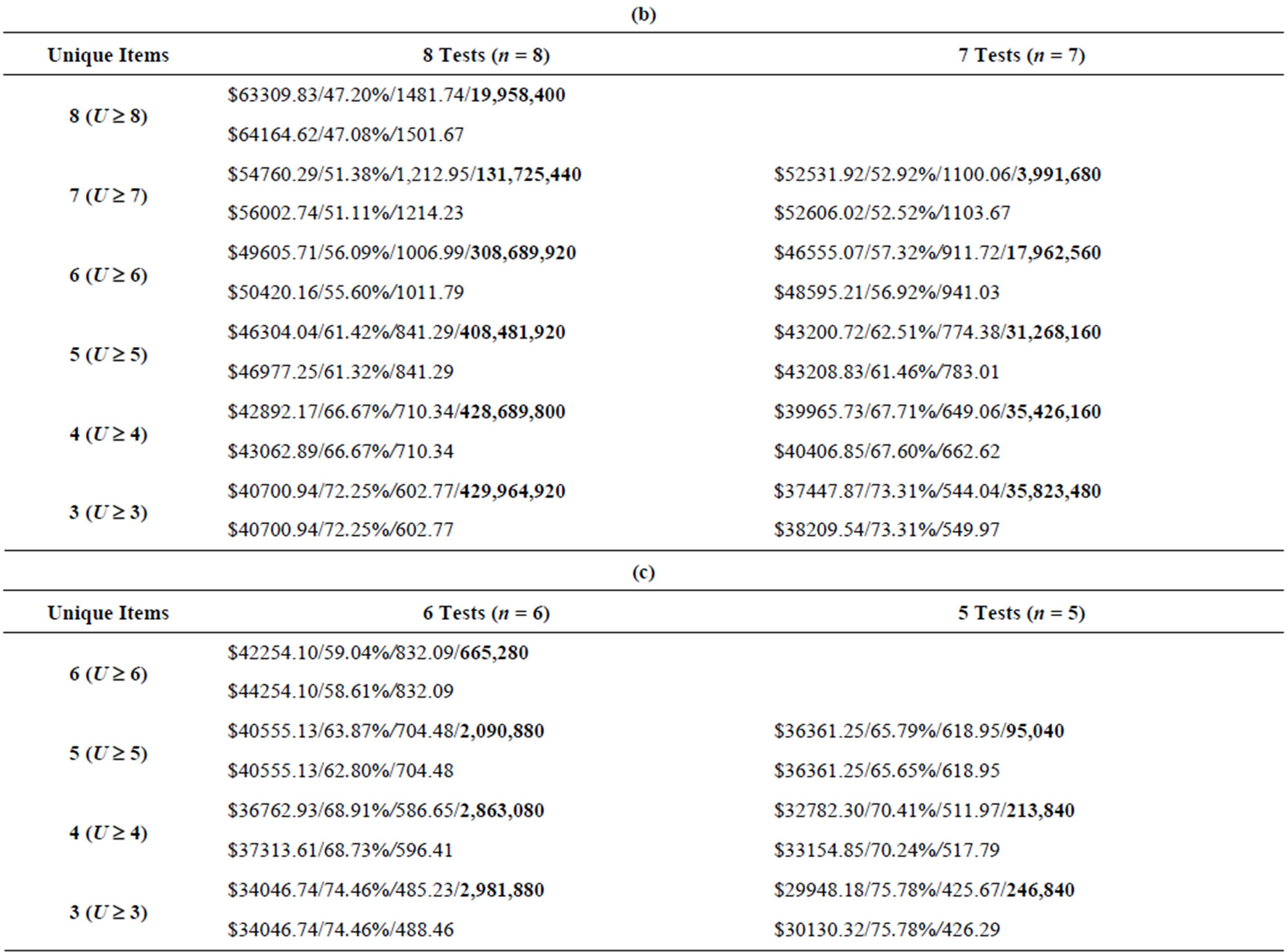
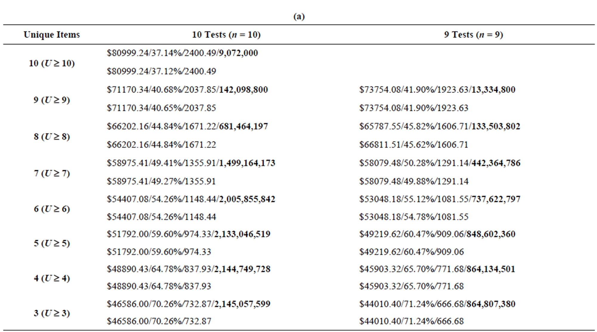
Table 11. (a) Results from input4 data set, 10 tests and 9 tests (m = 12); (b) Results from input4 data set, 8 tests and 7 tests (m = 12); (c) Results from input4 data set, 6 tests and 5 tests (m = 12).
Algorithm for this example problem, the last line of Table 12 shows the Relative Inferiority of the Genetic Algorithm, where the Relative Inferiority metrics were introduced via Equations (11)-(13).
For the hypothesis tests (H1 - H3), a summary is detailed in Table 13 below.
5.2. Discussion of Results
All three hypothesis tests show that the performance of the Genetic Algorithm is inferior to optimal results obtained via enumeration. As such, we are unable to claim that the Genetic Algorithm provides, from a statistical standpoint, optimal results.
However, the number of conforming units accepted through the nth inspection station (N(A|G)) metric shows inferiority of 1.73% compared to optimal, whereas total cost of the inspection plan (TC) and the ratio (Z) both show inferiority of less than 0.50%. The authors therefore consider the performance of the Genetic Algorithm formidable.
It should be noted that of the three performance measures shown above, the relative inferiority of the objective function value (Z) show the least relative inferiority, or stated another way, shows the most formidable result. This should not come as a surprise, considering the genetic algorithm was singularly motivated to find the lowest possible value of Z.
6. Concluding Comments
This effort presented a Genetic Algorithm approach to addressing the multiple-attribute inspection problem when multiple objectives are a concern. The literature has seen little work done for multiple inspection problems when multiple product attributes require inspection. As such, the authors felt compelled to address this relevant problem. Additionally, most work done for multiple inspection problems focuses on the objective of cost

Table 12. Solution detail for example problem.

Table 13. Hypothesis test results for test problems.
minimization. Given this, the authors also felt compelled to address maximization of conforming units surviving inspection in addition to cost minimization.
The authors felt compelled to address an objective in addition to cost minimization for the simple reason that cost minimization alone will favor all low-cost possibilities in terms of choosing attributes to be inspected as part of the inspection plan. The authors wanted to simultaneously consider a non-cost related performance measure, so that low-cost possibilities do not dominate the construction of the inspection plan. Maximization of conforming units surviving the final inspection station was considered a reasonable objective to pursue.
While the Genetic Algorithm approach did not provide optimal results, the results were still considered formidable, where the level of inferiority, in terms of the objective function (which considers both cost and conforming units accepted), obtained via the Genetic Algorithm, was less than 0.30%. The authors are comfortable in classifying this result as “near-optimal”.
Despite a formidable performance by the Genetic Algorithm, concerns remain. Past research has shown that heuristic performance, as compared to optimal performance, generally deteriorates to some degree as the problem size increases [18]. For this research, the largest problems encountered had been in excess of two billion feasible solutions. From a practical standpoint, it is difficult to enumerate all feasible solutions for problems larger than this. As such, gauging the performance of the Genetic Algorithm as compared to optimal performance is a challenge that remains. To compare this Genetic Algorithm’s performance to optimal performance for larger problems, improvements in CPU speed and memory capacity must come to fruition.
Another issue that requires mentioning relates to the objectives of cost minimization and maximization of conforming units surviving inspection. These two objectives were simultaneously considered via a ratio involving the two. This mathematical type of aggregation of the two objectives can certainly lead to a discussion regarding the best way to aggregate multiple objectives, and can start a debate on the best way to “scale” the objectives, “weight” the objectives and so on. This unresolved issue is considered as a future research opportunity.
Another future research opportunity relates to other objectives, aside from, or in addition to, the objectives addressed via this research effort. Cost minimization and maximization of conforming units surviving all inspection stations are not the only entities of importance. Even though the cost of sending a defective unit to the customer is factored into the total cost function, this concern could be directly addressed via an objective function component. Another entity that could be addressed is cost minimization on a per inspection basis. At present, the number of inspection stations to employ is pre-determined, or constrained. This need not be the case—a future research opportunity could explore cost minimization where the number of inspection stations need not be pre-determined, but be determined via the chosen search heuristic.
REFERENCES
- A. Tzimerman and Y. T. Herer, “Off-Line Inspections under Inspection Errors,” IIE Transactions, Vol. 41, No. 7, 2009, pp. 626-641. http://dx.doi.org/10.1080/07408170802331250
- G. D. Eppenand G. Hurst, “Optimal Location of Inspection Stations in a Multistage Production Process,” Management Science, Vol. 20, No. 8, 1974, pp. 1194-1200. http://dx.doi.org/10.1287/mnsc.20.8.1194
- T. Raz and M. Kaspi, “Location and Sequencing of Imperfect Inspection Operations Serial Multi-Stage Production Systems,” International Journal of Production Research, Vol. 8, No. 3, 1991, pp. 1645-1659.
- D. P. Ballou and H. L. Pazer, “The Impact of Inspector Fallibility on the Inspection Policy in Serial Production Systems,” Management Science, Vol. 28, No. 4, 1982, pp. 387-399.
- T. Raz and M. U. Thomas, “A Method for Sequencing Inspection Activities Subject to Errors,” IIE Transactions, Vol. 15, No. 1, 1983, pp. 12-18. http://dx.doi.org/10.1080/05695558308974608
- T. Raz and D. Bricker, “Sequencing of Imperfect Inspection Operations Subject to Constraints on the Quality of Accepted and Rejected Units,” International Journal of Production Research, Vol. 25, No. 6, 1987, pp. 809-821. http://dx.doi.org/10.1080/00207548708919878
- T. Raz and D. Bricker, “Optimal and Heuristic Solutions to the Variable Inspection Policy Problem,” Computers & Operations Research, Vol. 18, No. 1, 1991, pp. 115-123. http://dx.doi.org/10.1016/0305-0548(91)90047-U
- J. W. Schmidt and G. K. Bennett, “Economic multiattribute Acceptance Sampling,” AIIE Transactions, Vol. 4, No. 3, 1972, pp. 194-199.
- K. Tang, R. Plante and H. Moskowitz, “Multiattribute Bayesian Acceptance Sampling Plans under Non-Destructive Inspection,” Management Science, Vol. 32, No. 6, 1986, pp. 739-750. http://dx.doi.org/10.1287/mnsc.32.6.739
- K. Tang and J. Tang, “Design of Product Specifications for Multi-Characteristic Inspection,” Management Science, Vol. 35, No. 6, 1989, pp. 743-756. http://dx.doi.org/10.1287/mnsc.35.6.743
- L. L. Hau, “On the Optimality of a Simplified Multicharacteristic Component Inspection Model,” IIE Transactions, Vol. 20, No. 4, 1988, pp. 393-398.
- C. Shaoxiang and M. Lambrecht, “The Optimal Frequency and Sequencing of Tests in the Inspection of Multicharacteristic Components,” IIE Transactions, Vol. 29, No. 12, 1997, pp. 1039-1049. http://dx.doi.org/10.1080/07408179708966422
- T. Avinadav and D. Sarne, “Sequencing Counts: A Combined Approach for Sequencing and Selecting Costly Unreliable Off-Line Inspections,” Computers & Operations Research, Vol. 39, No. 11, 2012, pp. 2488-2499. http://dx.doi.org/10.1016/j.cor.2011.12.018
- T. Raz and D. Bricker, “Sequencing of Inspection Operations Subject to Errors,” European Journal of Operational Research, Vol. 68, No. 2, 1993, pp. 251-264. http://dx.doi.org/10.1016/0377-2217(93)90307-9
- J. S. Park, M. H. Peters and K. Tang, “Optimal Inspection Policy in Sequential Screening,” Management Science, Vol. 37, No. 8, 1991, pp. 1058-1061. http://dx.doi.org/10.1287/mnsc.37.8.1058
- D. E. Goldberg, “Genetic Algorithms in Search, Optimization and Machine Learning,” Addison-Wesley, Reading, 1989.
- Z. Michelawicz and D. Fogel, “How to Solve It: Modern Heuristics,” Springer, New York, 2010.
- P. R. McMullen, “JIT Mixed-Model Sequencing with Batching and Setup Considerations via Search Heuristics,” International Journal of Production Research, Vol. 48, No. 22, 2010, pp. 6559-6582. http://dx.doi.org/10.1080/00207540903321640