Int'l J. of Communications, Network and System Sciences
Vol.2 No.2(2009), Article ID:423,4 pages DOI:10.4236/ijcns.2009.22012
MATLAB Simulink Simulation Platform for Photonic Transmission Systems
Centre for Telecommunications and Information Engineering, Department of Electrical
and Computer Systems Engineering, Monash University, Clayton Campus, Clayton Victoria, Australia
Email: le.nguyen.binh@eng.monash.edu.au
Received October 25, 2008; revised December 20, 2008; accepted December 31, 2008
Keywords: Communications Systems, MATLAB Simulink Simulation, Optical Communications
Abstract
High speed and ultra-high capacity optical communications have emerged as the essential techniques for backbone global information transmission networks. As the bit rate of the transmission system gets higher and higher 40 Gb/s to 100 Gb/s the modeling of proposed modulation techniques is very important so as to avoid costly practical demonstration. The search for a universal modeling platform for such systems is urgent. Matlab Simulink has become the universal mathematical and modeling tools in most universities and research laboratories around the world. This paper thus describes the modeling techniques for advanced photonic transmission systems and Simulink is proven to be very effective platform for development of photonic communications systems due its comprehensive blocksets. The simulation is based mainly on the physical phenomena and understanding of its concepts of communications and photonics. Simulink models are given as examples of various sub-systems of the photonic transmission systems. Some simulated transmission performances are demonstrated as examples of final results obtained from Simulink models of the transmission systems.
1. Introduction
1.1. Overview of a Digital Photonic System
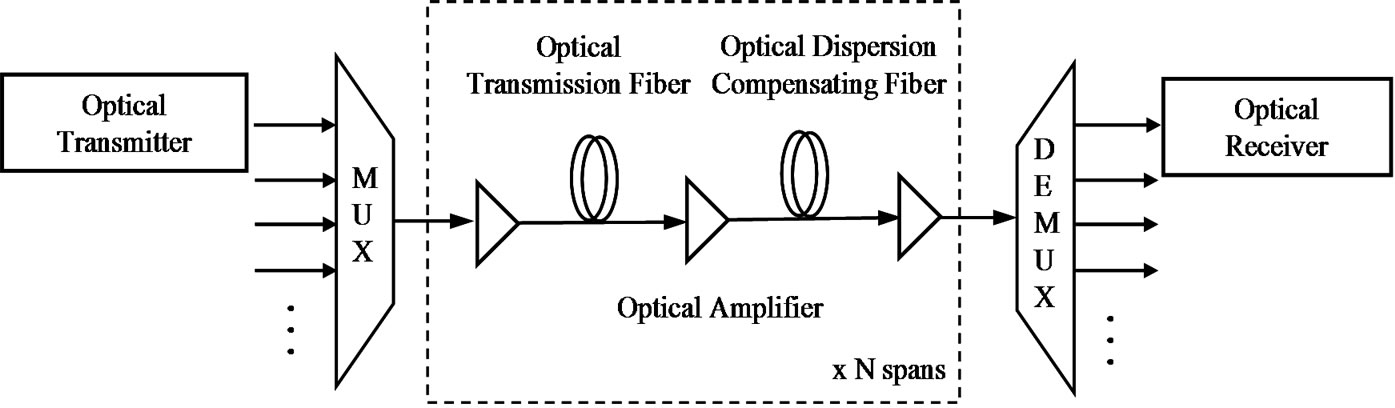
Any study on digital photonic transmission systems requires in-depth understanding of operational principles of system components which involve: 1) modulation/ demodulation or generation/detection of the optical signals modulated by proposed formats and the detection here implies the incoherent direct detection; 2) impairments in either electronic or photonic domains, especially the dynamics of optical fiber and the noise sources contributed by optical amplifiers and receiver electronic noise; 3) effects of optical and electrical filters. The schematic diagram of a DWDM digital photonic system is illustrated in Figure 1.
The transmission medium may consist a variety of fiber types such as the standard SMF ITU-G.652 or nonzero dispersion shifted fibers (NZ-DSF) ITU-G.655 or the new type of fiber: Corning Vascade fiber. The dispersion and distortion of the lightwave signals are usually compensated by dispersion compensating fibers (DCF). The DCFs are normally accompanied by two discrete optical amplifiers, the Erbium-doped optical amplifiers (EDFA), one is for pre-amplification to compensate the attenuation of the transmission span, and the other is a booster amplifier for boosting the optical power of the channels to an acceptable, below the nonlinear limit level. It is assumed in this work that the amplifiers are operating in the saturation region.
The receiving sub-system would take on: 1) single detector direct detection optical receiver 2) the balanced detector receiving structure. The first type of the receiver is widely used for detection of ASK modulated optical signals. For the later case, the structure acts as an optical phase comparator employing a delay interferometer. Detailed description of these direct detection receivers for novel modulation formats are presented. In addition, especially for contemporary systems with high capacity, high bit rate and requiring high performance, electronic equalizers can be employed as part of the receiver. Section 5 gives insight and performance of one of the most effective electronic equalizers which is maximum likelihood sequence estimation (MLSE) with Viterbi algorithm.
1.2. Matlab Simulink® Modeling Platform
High speed and high capacity modern digital photonic systems require careful investigations on the theoretical performance against various impairments caused by either electronics or fiber dynamics before they are deployed in practice. Thus, the demand for a comprehensive modeling platform of photonic systems is criticalespecially a modeling platform that can structure truly the photonic sub-systems. A simulation test-bed is necessary for detailed design, investigation and verification on the benefits and shortcomings of these advanced modulation formats on the fiber-optic transmission systems Furthermore the modeling platform should take advantage of any user-friendly software platform that are popular and easy for use and further development for all the operators without requiring very much expertise in the physics of the photonic systems. Besides, this platform would offer research community of optical communication engineering a basis for extension and enhance the linkages between research groups.
 (a)
(a) (b)
(b)
Figure 1. (a) General block diagram of the DWDM optical fiber transmission system. (b) MATLAB Simulink model.
Thus, it is the principal incentive for the development of a simulation package based on Matlab Simulink® platform1 To the best of my knowledge, this is the first Matlab© Simulink-platform photonic transmission testbed for modeling advanced high capacity and long-haul digital optical fiber transmission systems. The simulator is used mainly for investigation of performance of advanced modulation formats, especially the amplitude and/or phase shift keying modulation with or without the continuity at the phase transition. Here, a single channel optical system is of main interest for implementation of the modeling in this paper.
Several noticeable advantages of the developed Matlab Simulink®modeling platform are listed as follows:
•The simulator provides toolboxes and blocksets adequately for setting up any complicated system configurations under test. The initialization process at the start of any simulation for all parameters of system components can be automatically conducted. The initialization file is written in a separate Matlab file so that the simulation parameter can be modified easily.
•Signal monitoring is especially easy to be carried out. Signals can be easily monitored at any point along the propagation path in a simulation with simple plug-and-see monitoring scopes provided by Simulink®.
•Numerical data including any simulation parameters and the numerical results can be easily stored for later processing using Matlab toolboxes. This offers a complete package from generating the numerical data to processing these data for the achievement of final results.
•A novel modified fiber propagation algorithm has been developed and optimized to minimize the simulation processing time and enhance its accuracy.
•The transmission performance of the optical transmission systems can be automatically and accurately evaluated with various evaluation methods. These methods, especially proposal of novel statistical evaluation techniques are to be presented in Section 6.
Several Matlab Simulink® modeling frameworks are demonstrated in the Appendix of this paper. A Simulink model of a photonic transmission system can be shown in Figure 1(b).
2.Optical Transmitters
The transmitters would consist of a narrow linewidth laser source to generate lightwaves of wavelength conformed to the ITU grid. These lightwaves are combined and then modulated. This form is for laboratory experiments only. In practice each laser source would be modulated by an external modulation sub-system. The MZIM can bee a single or dual drive type. The schematic of the modulator is shown in Figure 2(a) and the Simulink model is in Figure 2(a) for generation of photonic signals by multi-level amplitude and phase shift keying modulation formats.
In 1980s and 1990s, direct modulation of semiconductor lasers was the choice for low capacity coherent optical systems over short transmission distance. However, direct modulation induces chirping which results in severe dispersion penalties. In addition, laser phase noise and induced from non-zero laser linewidth also limit the advance of direct modulation to higher capacity and higher bit rate transmission.
Overcoming the mentioned issues, external modulation techniques have been the preferred option for digital photonic systems for over the last decade. External modulation can be implemented using either electro-absorption modulator or electro-optic modulators (EOM). The EOM whose operation is based on the principles of electro-optic effect (i.e. change of refractive index in solid state or polymeric or semiconductor material is proportional to the applied electric field) has been the preferred choice of technology due to better performance in terms of chirp, extinction ratio and modulation speed. Over the years, the waveguides of the electrooptic modulators are mainly integrated on the material platform of lithium niobate (LiNbO3) which has been the choice due to their prominent properties of low loss, ease of fabrication and high efficiency [4].
These LiNbO3 modulators have been developed in the early 1980s, but not popular until the advent of the Erbium-doped optical fiber amplifier (EDFA) in the late 1980s. Prior to the current employment of LiNbO3 modulators for advanced modulation formats, they were employed in coherent optical communications to mitigate the effects of broad linewidth due to direct modulation of the laser source. These knowledges have recently been applied to the in-coherent advanced modulation formats for optically amplified transmission systems.
EOMs are utilized for modulation of either the phase or the intensity of the lightwave carrier. The later type is a combination of two electro-optic phase modulators (EOPMs) forming an interferometric configuration.
2.1. Optical Phase Modulator
Electro-optic phase modulator employs a single electrode as shown in Figure 3. When a RF driving voltage is applied onto the electrode, the refractive index changes accordingly inducing variation amount of delays of the propagating lightwave. Since the delays correspond to the phase changes, EOPM is used to carry out the phase modulation of the optical carrier.
 (a)
(a)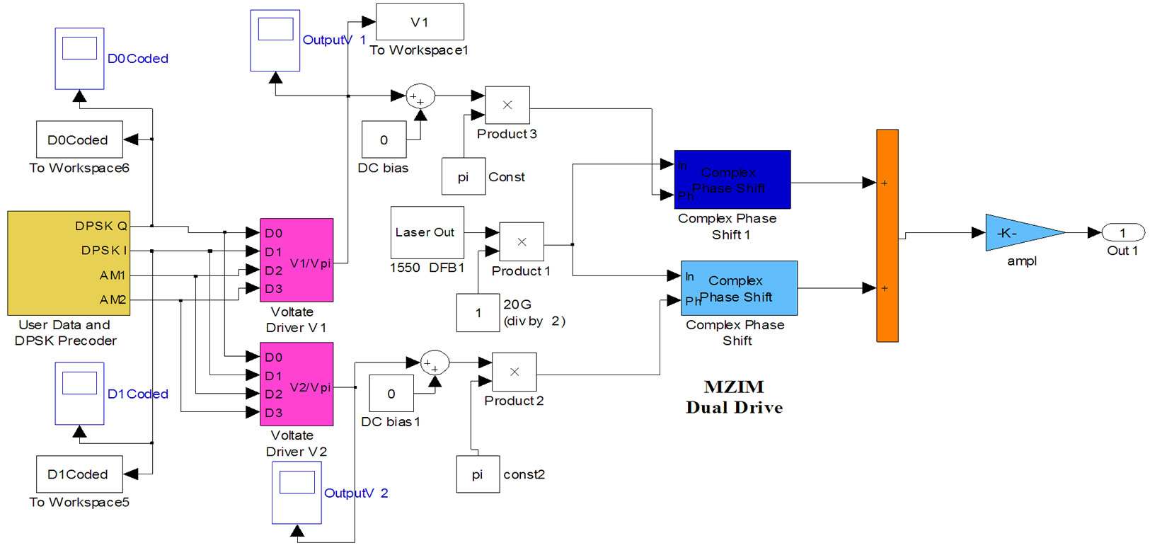 (b)
(b) (c)
(c)
Figure 2. Structure of external modulation for generation of advanced modulation format lightwave signals. (a) Schematic. (b) Simulink model of pre-coder and modulation. (c) Details of MZIM.
The induced phase variation is governed by the following equation:
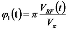 (1)
(1)
where Vπ is the RF driving voltage required to create a π phase shift of the lightwave carrier and typically has a value within a range of 3V to 6V. The optical field at the output of an EOPM is generated given in following equation:
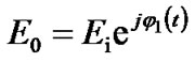 (2)
(2)
where Eo is the transmitted optical field at the output the MZIM and noted in the low pass equivalent representation i.e the carrier is removed from the expression; V(t) is the time-varying signal voltage, Vbias is the DC bias voltage applied to the phase modulator.
Recently, EOPMs operating at high frequency using resonant-type electrodes have been studied and proposed in [2,3]. Together with the advent of high-speed electronics which has evolved with the ASIC technology using 0.1µm GaAs P-HEMT or InP HEMTs [4], the contemporary EOPMs can now exceed 40Gb/s operating rate without much difficulty.
Such phase modulation can be implemented in MATLAB Simulink as shown in Figure 2(b) using a phase shift block of the Common Blockset. The phase bias is in one phase shift block and then the signal modulation or time dependent is fed into another phase shift block. The signals of the two parallel phase shift/modulation blocks are then combined to represent the interferometric construction and destruction, thus an intensity modulation can be achieved as described in the next sub-section.
2.2. Optical Intensity Modulator
Optical intensity modulation is operating based on the principle of interference of the optical field of the two lightwave components. A LiNbO3 optical intensity modulator thus employs the interferometric structure as
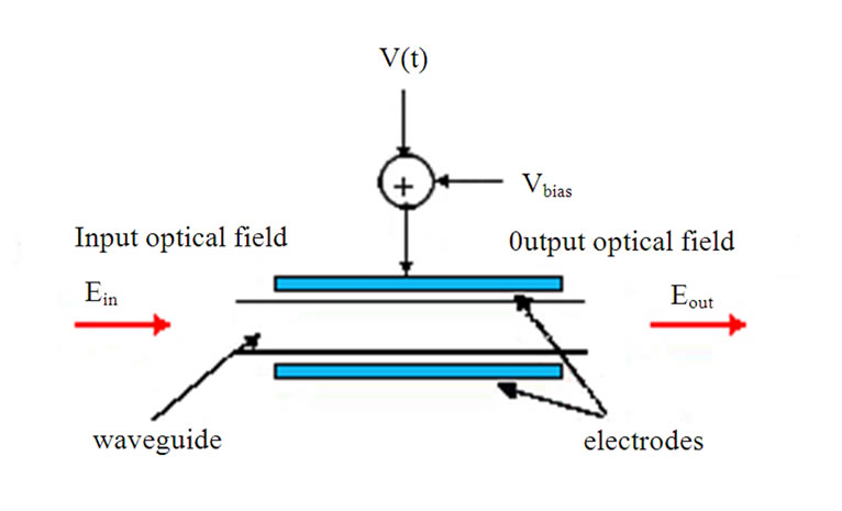
Figure 3. Electro-optic optical phase modulator.
shown in Figure 4 and is most popularly well-known as the Mach-Zehnder interferometer (MZIM). The operational principles are briefly explained in the following paragraph. For the rest of the chapters in this paper, unless specifically indicated, the term of optical modulator is referred to the external LiNbO3 MZIM modulator.
The lightwave is split into two arms when entering the modulator. The power slitter is normally a 3-dB type i.e equally splitting the power of the optical signals. Each arm of the LiNbO3 modulator employs an electro-optic phase modulator in order to manipulate the phase of the optical carrier if required. At the output of the MZIM, the lightwaves of the two arm phase modulators are coupled and interfered with each other. The transfer curve of an MZIM is shown in Figure 4(c). A LiNbO3 MZIM modulator can be a single or dual drive type.
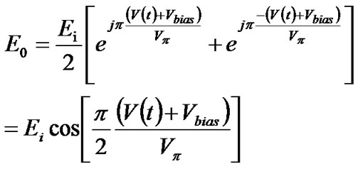
In the case of single-drive MZIM, there is only a single RF voltage driving one arm of the MZIM. For instance, there is no RF driving voltage on arm 1, hence V1(t) = 1 and the RF voltage V2(t) applied on arm 2 is noted as V(t). The transmitted optical field E(t) at the output a single-drive MZIM as a function of the driving voltage V(t) and a bias DC voltages Vbias can be written as
 (3)
(3)
where Vπ. is the required driving voltage to obtain a π phase shift in the lightwave carrier.
It can be seen that the phase term in Equation (1) implies the existence of the modulation of the optical carrier phase and commonly known as the chirping effect. Thus, by using a single-drive MZIM, generated optical signals is not chirp-free. Furthermore, it is reported that a z-cut LiNbO3 MZIM can provide a modest amount of chirping due to its asymmetrical structure of the electrical field distributions whereas its counterpart x-cut

Figure 4. Optical intensity modulator based on MachZehnder interferometric structure.
MZIM is a chirp-free modulator thanks to the symmetrical or push-pull configuration of the electrical fields. Furthermore, also having a push-pull arrangement, complete elimination of chirping effect in modulation of the lightwave can be implemented with use of a dual-drive MZIM. The transmitted optical field E(t) at the output a MZIM as a function of the driving and bias voltages can be written as
 (4)
(4)
In a dual-drive MZIM, the RF driving voltage V1(t) and V2(t) are inverse with each other i.e V2(t)=-V1(t). Equation (4) indicates that there is no longer phase modulation component, hence the chirping effect is totally eliminated.
3. Fiber Transmission Dynamics
3.1. Chromatic Dispersion (CD)
This section briefly presents the key theoretical concepts describing the properties of chromatic dispersion in a single-mode fiber. Another aim of this section is to introduce the key parameters which will be commonly mentioned in the rest of the paper.
The initial point when mentioning to the chromatic dispersion is the expansion of the mode propagation constant or “wave number” parameter, β, using the Taylor series:
 (5)
(5)
where ω is the angular optical frequency, n(ω) is the frequency-dependent refractive index of the fiber. The parameters 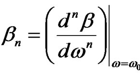 have different physical meanings as 1) βo is involved in the phase velocity of the optical carrier which is defined as
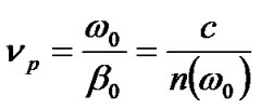 ; 2) β1determines the group velocity νg which is related to the mode propagation constant β of the guided mode by [5,6]
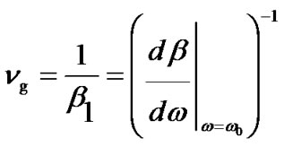 (6)
(6)
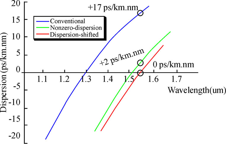
Figure 5. Typical values of dispersion factor for different types of fiber.
And 3) β2 is the derivative of group velocity with respect to frequency. Hence, it clearly shows the frequency-dependence of the group velocity. This means that different frequency components of an optical pulse travel at different velocities, hence leading to the spreading of the pulse or known as the dispersion. β2 is therefore is known as the famous group velocity dispersion (GVD). The fiber is said to exhibit normal dispersion for β2>0 or anomalous dispersion if β2<0.
A pulse having the spectral width of  is broadened by
 . In practice, a more commonly used factor to represent the chromatic dispersion of a single mode optical fiber is known as D (ps/nm.km). The dispersion factor is closely related to the GVD β2 and given by:
 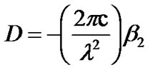 at the operating wavelength λ; where β3 defined as
 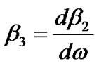 contributes to the calculations of the dispersion slope,
  , which is an essential dispersion factor for high-speed DWDM transmission.
  can be obtained from the higher order derivatives of the propagation constant as
 (7)
(7)
A well-known parameter to govern the effects of chromatic dispersion imposing on the transmission length of an optical system is known as the dispersion length LD. Conventionally, the dispersion length LD corresponds to the distance after which a pulse has broadened by one bit interval. For high capacity long-haul transmission employing external modulation, the dispersion limit can be estimated in the following Equation [8].
 (8)
(8)
where B is the bit rate (Gb/s), D is the dispersion factor (ps/nm km) and LD is in km.
Equation (8) provides a reasonable approximation even though the accurate computation of this limit that depends the modulation format, the pulse shaping and the optical receiver design. It can be seen clearly from (8) that the severity of the effects caused by the fiber chromatic dispersion on externally modulated optical signals is inversely proportional to the square of the bit rate. Thus, for 10 Gb/s OC-192 optical transmission on a standard single mode fiber (SSMF) medium which has a dispersion of about ±17 ps/nm.km, the dispersion length LD has a value of approximately 60 km i.e corresponding to a residual dispersion of about ±1000 ps/nm and less than 4 km or equivalently to about ± 60 ps/nm in the case of 40Gb/s OC-768 optical systems. These lengths are a great deal smaller than the length limited by ASE noise accumulation. The chromatic dispersion therefore, becomes the one of the most critical constraints for the modern high-capacity and ultra long-haul transmission optical systems.
3.2. Polarization Mode Dispersion (PMD)
Polarization mode dispersion (PMD) represents another type of the pulse spreading. The PMD is caused by the
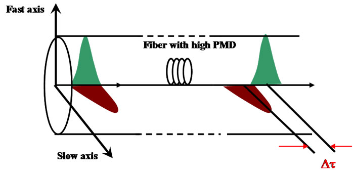
Figure 6. Demonstration of delay between two polarization states when lightwave propagating optical fiber.
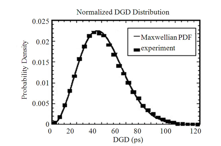
Figure 7. The Maxwellian distribution is governed by the following expression: Equation (9).
differential group delay (DGD) between two principle orthogonal states of polarization (PSP) of the propagating optical field.
One of the intrinsic causes of PMD is due to the asymmetry of the fiber core. The other causes are derived from the deformation of the fiber including stress applied on the fiber, the aging of the fiber, the variation of temperature over time or effects from a vibration source. These processes are random resulting in the dynamic of PMD. The imperfection of the core or deformation of the fiber may be inherent from the manufacturing process or as a result of mechanical stress on the deployed fiber resulting in a dynamic aspect of PMD.
The delay between these two PSP is normally negligibly small in 10Gb/s optical transmission systems. However, at high transmission bit rate for long-haul and ultra long-haul optical systems, the PMD effect becomes much more severe and degrades the system performance [9-12]. The DGD value varies along the fiber following a stochastic process. It is proven that these DGD values complies with a Maxwellian distribution as shown in Figure 7 [10,13,14].
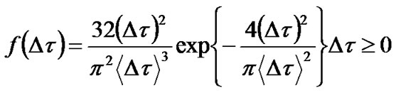 (9)
(9)
where  is differential group delay over a segment of the optical fiber
 . The mean DGD value
  is commonly termed as the “fiber PMD” and normally given by the fiber manufacturer.
An estimate of the transmission limit due to PMD effect is given as:
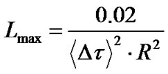 (10)
(10)
where R is the transmission bit rate. Therefore,  =1 ps/km (older fiber vintages); Bit rate = 40 Gbit/s; Lmax=12.5 Km; Bit rate =10 Gbit/s; Lmax=200 Km;
  =0.1 ps/km (contemporary fiber for modern optical systems); Bit rate = 40 Gbit/s; Lmax=1250 Km ; thence for Bit rate = 10 Gbit/s ; Lmax=20.000 Km.
Thus PMD is an important impairment of ultra long distance transmission system even at 10 Gb/s optical transmission. Upgrading to higher bit rate and higher capacity, PMD together with CD become the most two critical impairments imposing on the limitation of the optical systems.
3.3. Fiber Nonlinearity
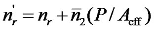
The fiber refractive index is not only dependent of wavelength but also of intensity of the lightwave. This well-known phenomenon which is named as the Kerr effect is normally referred as the fiber nonlinearity. The power dependence of the refractive index nr is shown in the following expression
 (11)
(11)
P is the average optical intensity inside the fiber,  is the nonlinear-index coefficient and Aeff is the effective area of the fiber.
There are several non-linearity phenomena induced from the Kerr effects including intra-channel self-phase modulation (SPM), cross phase modulation between inter-channels (XPM). four wave mixing (FWM), stimulated Raman scattering (SRS) and stimulated Brillouin scattering (SBS). SRS and SBS are not main degrading factors compared to the others. FWM effect degrades performance of an optical system severely if the local phase of the propagating channels are matched with the introduction of the ghost pulse. However, with high local dispersion parameter such as in SSMF or even in NZDSF, effect of the FWM becomes negligible. XPM is strongly dependent on the channel spacing between the channels and also on local dispersion factor of the optical fiber [refs]. [ref] also report about the negligible effects of XPM on the optical signal compared the SPM effect. Furthermore, XPM can be considered to be negligible in a DWDM system in the following scenarios: 1) highly locally dispersive system e.g SSMF and DCF deployed systems; 2) large channel spacing and 3) high spectral efficiency [15-19]. However, the XPM should be taken in to account for the systems deploying Non-zero dispersion shifted fiber (NZ-DSF) where the local dispersion factor is low. The values of the NZ-DSF dispersion factors can be obtained from Figure 5. Among nonlinearity impairments, SPM is considered to be the major shortfalls in the system.
In this paper, only the SPM non-linearity is generally considered. This is the main degradation factor for high bit rate transmission system where the signal spectrum is broadened. The effect of SPM is normally coupled with the nonlinear phase shift which is defined as
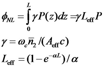 (12)
(12)
where wc is the lightwave carrier, Leff is the effective transmission length and α is the attenuation factor of a SSMF which normally has a value of 0.17-0.2 dB/km for the currently operating wavelengths within the 1550nm window. The temporal variation of the non-linear phase fNL while the optical pulses propagating along the fiber results in the generation of new spectral components far apart from the lightwave carrier wc implying the broadening of the signal spectrum. The spectral broadening dw which is well-known as frequency chirping can be explained based on the time dependence of the nonlinear phase shift and given by the expression:
 (13)
(13)
From (13), the amount of dw is proportional to the time derivative of the signal power P. Correspondingly, the generation of new spectral components may mainly occur the rising and falling edges of the optical pulse shapes, i.e. the amount of generated chirp is larger for an increased steepness of the pulse edges.
4. Modeling of Fiber Propagation
4.1 Non-linear Schrodinger Equation (NLSE)
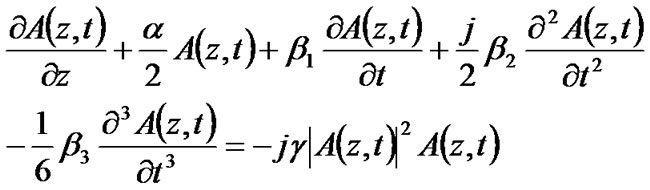
Evolution of the slow varying complex envelope A(z,t) of the optical pulses along a single mode optical fiber is governed by the well-known nonlinear Schroedinger equation (NLSE):
 (14)
(14)
where z is the spatial longitudinal coordinate, α accounts for fiber attenuation,  indicates the differential group delay (DGD),
  and
and  represent 2nd and 3rd order factors of the group velocity dispersion (GVD) and
  is the nonlinear coefficient. Equation (14) involves the following effects in a single-channel transmission fiber: 1) the attenuation, 2) chromatic dispersion, 3) 3rd order dispersion factor i.e the dispersion slope, and 4) self phase modulation nonlinearity. Other critical degradation factors such as the non-linear phase noise due to the fluctuation of the optical intensity caused by ASE noise via Gordon-Mollenauer effect [20] is mutually included in the equation.
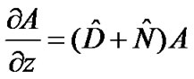
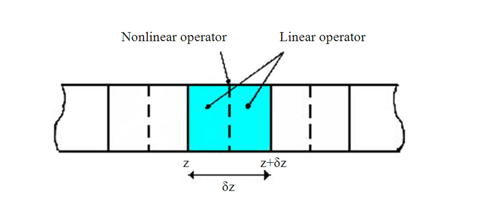
4.2. Symmetrical Split Step Fourier Method
In this Paper, solutions of the NLSE and hence the model of pulse propagation in a single mode optical fiber is numerically solved by using the popular approach of the split step Fourier method (SSFM) [5] in which the fiber length is divided into a large number of segments of small step size .
.
In practice, dispersion and nonlinearity are mutually interactive while the optical pulses propagate through the fiber. However, the SSFM assumes that over a small length , the effects of dispersion and the nonlinearity on the propagating optical field are independent. Thus, in SSFM, the linear operator representing the effects of fiber dispersion and attenuation and the nonlinearity operator taking into account fiber nonlinearities are defined separately as
 (15)
(15)
where A replace s for simpler notation and T=t-z/vg is the reference time frame moving at the group velocity. The NLSE Equation (14) can be rewritten as
 (16)
(16)
and the complex amplitudes of optical pulses propagating from z to z+  is calculated using the approximation as given:
 (17)
(17)
Equation (14) is accurate to second order in the step size . The accuracy of SSFM can be improved by including the effect of the nonlinearity in the middle of the segment rather than at the segment boundary as illustrated in Equation (17) can now modified as
 (a)
(a) (b)
(b)
Figure 8. (a) Schematic illustration of the split-step Fourier method. (b) MATLAB Simulink model.

This method is accurate to third order in the step size . The optical pulse is propagated down segment from segment in two stages at each step. First, the optical pulse propagates through the first linear operator (step of
  /2) with dispersion effects taken into account only. The nonlinearity is calculated in the middle of the segment. It is noted that the nonlinearity effects is considered as over the whole segment. Then at z+
 /2, the pulse propagates through the remaining
  /2 distance of the linear operator. The process continues repetitively in executive segments
  until the end of the fiber. This method requires the careful selection of step sizes
  to reserve the required accuracy.
The Simulink model of the lightwave signals propagation through optical fiber is shown in Figure 8(b). All parameters required for the propagation model are fed as the inputs into the block. The propagation algorithm split-steps and FFT are written in .m files in order to simplify the model. This demonstrates the effectiveness of the linkage between MATLAB and Simulink. A Matlab program is used for modeling of the propagation of the guided lightwave signals over very long distance is given in the Appendix.
4.3. Modeling of Polarization Mode Dispersion (PMD)
The first order PMD effect can be implemented by splitting the optical field into two distinct paths representing two states of polarizations with different propagating delays , then implementing SSFM over the segment
  before superimposing the outputs of these two paths for the output optical field.
The transfer function for first-order PMD is given by [21].
 (19)
(19)
 and
and
with  is the splitting ratio. The usual assumption is
  =1/2. Finite impulse response filter blocks of the digital signal processing blocksets of Simulink can be applied here without much difficulty to represent the PMD effects with appropriate delay difference.
4.4. Fiber Propagation in Linear Domain
Here, the low pass equivalent frequency response of the optical fiber, noted as H(f) has a parabolic phase profile and can be modeled by the following equation, [22]
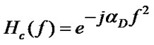 (20)
(20)
where,  represents the Group Velocity Distortion (GVD) parameter of the fiber and L is the length of the fiber. The parabolic phase profile is the result of the chromatic dispersion of the optical fiber [23]. The 3rd order dispersion factor b3 is not considered in this transfer function of the fiber due to negligible effects on 40Gb/s transmission systems. However, if the transmission bit rate is higher than 40Gb/s, the b3 should be taken into account.
In the model of the optical fiber, it is assumed that the signal is propagating in the linear domain, i.e. the fiber nonlinearities are not included in the model. These nonlinear effects are investigated numerically. It is also assumed that the optical carrier has a line spectrum. This is a valid assumption considering the stateof-the-art laser sources nowadays with very narrow linewidth and the use of external modulators in signal transmission.
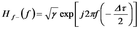
A pure sinusoidal signal of frequency f, propagating through the optical fiber, experiences a delay of |2πfDb2L|. The standard fibers used in optical communications have a negative  and thus, in low pass equivalent representation, sinusoids with positive frequencies (i.e. frequencies higher than the carrier) have negative delays, i.e. arrive early compared to the carrier and the ones with negative frequencies (i.e. frequencies lower than the carrier) have positive delays and arrive delayed. The dispersion compensating fibers have positive
  and so have reverse effects. The low pass equivalent channel impulse response of the optical fiber,
  has also followed a parabolic phase profile and is given as,
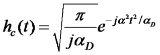 (21)
(21)
5. Optical Amplifier
5.1. ASE Noise of Optical Amplifier
The following formulation accounts for all noise terms that can be treated as Gaussian noise
 (22)
(22)
G =amplifier gain; nsp = spontaneous emission factor; m =number of polarization modes (1 or 2); PN =mean noise in bandwidth; OSNR at the output of EDFA.

Figure 9. Simulink model of an optical amplifier with gain and NF.
5.2. Optical Amplifier Noise Figure
Amplifier Noise Figure (NF) is defined at the output of the optical amplifier as the ratio between the output OSNR on the OSNR at the input of the EDFA.
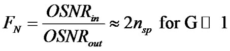 (23)
(23)
A Simulink model of the optical amplifier is shown in that represents all the system operational parameters of such amplifier. Only blocks of the Common Blockset of Simulink are used.
6. Optical Filter
In this paper, optical filtering of the noise-corrupted optical signals is conducted with a Gaussian-type filter whose 3dB bandwidth is governed by
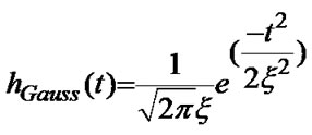 (24)
(24)
where 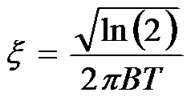 in which B is the Gaussian filter’s 3-dB bandwidth and T is the bit rate. The BT product parameter is B times the input signal’s bit period.
The modeling of an electrical filter can also use a Gaussian filter with similar impulse response as defined in (24) or a conventional analog 5th order Bessel filter which can be easily designed using filter design toolbox in Matlab. The Matlab pseudo-codes for designing an analog 5th order Bessel filter are shown as follows:
[b,a] = besself(5thorder,2*pi*BTb/os_fac); %Analog filter
[bz,az] = impinvar(b,a,1); %Digital filter
[hf t1] = impz(bz,az,2*delay*os_fac+1,os_fac);
In the above pseudo-codes, the BT product parameter is defined similarly to that in the case of a Gaussian filter. Alternatively, the transfer function of an analog 5th order Bessel filter can be referred from [24].
7. Optical Receiver
The demodulation of the original message is carried out in electrical domain, thus the conversion of lightwaves to electrical signals is required. In digital optical communication, this process has been widely implemented with a PIN photodiode in a coherent or incoherent detection. The first type requires a local oscillator to coherently down-convert the modulated lightwave from optical frequency to IF frequency. The second type which has been the preferred choice for currently deployed systems is the incoherent detection which is based on square-law envelop detection of the optical signals. For incoherent detection, the recovery of clock timing is critical. In the rest of this Paper and in the simulations, ideal clock timing is assumed.
After detection, the electrical current is normally amplified with a trans-impedance amplifier before passing through an electrical filter which is normally of Bessel type. The bandwidth of the electrical filter generally varies between 0.6 and 0.8 R. At this point, electrical eye diagrams are normally observed for the assessment of signal quality. Sampling of electrically filtered received signals is next carried out. Without use of electronic equalizers, hard decision which compares the received signal level to a pre-set threshold for making the decision is implemented.
For advanced phase modulation formats such as DPSK, CPFSK or MSK, a MZDI-based balanced receiver with two photodiodes connected back-to-back is required. Excluding the distortions of waveform due to fiber dynamics and from the analytical point of view, the received electrical signals are corrupted with noise from several sources including 1) shot noise ( ), 2) electronic noise
  of trans-impedance amplifier, 3) dark current noise
  and 4) interactions between signals and ASE noise (
 ) and between ASE noise itself
  as
as
 (25)
(25)
These noise sources are usually modeled with normal distributions whose variances representing the noise power are defined as
1) Shot noise is caused by the intrinsic electro-optic phenomenon of the semiconductor photodiode in which a random number of electron-hole pairs is generated with the receipt of photons causing the randomness of the induced photo-current. The shot noise is given in the following formula:
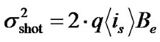 (26)
(26)
where Be is the 3dB bandwidth of the electrical filter, < is> is the average signal-only photo-current after the photodiodes.
2) The electronic noise source  is injected from the trans-impedance amplifier. It is modeled with an equivalent noise current density iNeq over the bandwidth of the electrical filter. The unit of iNeq is A/
 and the value of
  is obtained as (iNeq) 2Be.
3) Value of dark current idark is normally specified with a particular photo-diode and has the unit of A/Hz. Hence, the noise power  is calculated as idark Be.
4) The variances of amplitude fluctuations due to the beating of signal and ASE noise and between ASE noise itself are governed by the following expressions:
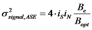 (27)
(27)
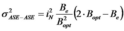 (28)
(28)
where Bopt is the 3dB bandwidth of the optical filter and iN is the noise-induced photo-current. In practice, the value of  is normally negligible compared to the value of
  and can be ignored without affecting the performance of the receiver.
It is worth noting that in an optically pre-amplified receiver, i.e. the optical signal is amplified at a stage before the photo-detector,  is the dominant factor compared to other noise sources.
8. Performance Evaluation
Performance evaluation of an optical transmission system via the quality of the electrically detected signals is an essential aspect in both simulation and experiment scenarios. The key metrics reflecting the signal quality include optical signal to noise ratio (OSNR) and OSNR penalty, eye opening (EO) and eye opening penalty (EOP) where as bit error rate (BER) is the ultimate indicator for the performance of a system.
In an experimental set-up and practical optical systems, BER and the quality factor Q-factor can be obtained directly from the modern BERT test-sets and data can be exported to a portable memory for post-processing. However, it is noted that these experimental systems need to be run within at least a few hours so that the results are stable and accurate.
For the case of investigation of performance of an optical transmission system by simulation, several methods have been developed such as
1) Monte Carlo numerical method
2) Conventional method to calculate Q-factor, Q dB and hence BER based on assumption of Gaussian distribution of noise.
3) Methods based on statistical processes taking into account the distortion from the dynamic effects of the optical fibers including the ISI induced by CD, PMD and tight optical filtering.
•The first statistical technique implements the Expected Maximization theory in which the pdf of the obtained electrical detected signal is approximated as a mixture of multiple Gaussian distributions.
•The second technique is based on the Generalized Extreme Values theorem. Although this theorem is wellknown in other fields such as financial forecasting, meteorology, material engineering, etc to predict the probability of occurrence of extreme values, it has not much studied to be applied in optical communications.
8.1. Monte Carlo Method
Similar to the bit error rate test (BERT) equipment commonly used in experimental transmission, the BER in a simulation of a particular system configuration can be counted. The BER is the ratio of the occurrence of errors (Nerror) to the total number of transmitted bits Ntotal and given as:
 (29)
(29)
Monte Carlo method offers a precise picture via the BER metric for all modulation formats and receiver types. The optical system configuration under a simula-

Figure 10. Simulink model of an optical balanced receiver.
tion test needs to include all the sources of impairments imposing to signal waveforms including the fiber impairments and ASE (optical)/electronic noise.
It can be seen that a sufficient number of transmitted bits for a certain BER is required and leading to exhaustive computational time. In addition, time-consuming algorithms such as FFT especially carried out in symmetrical SSFM really contribute to the long computational time. A BER of 1e-9 which is considered as ’error free’ in most scientific publications requires a number of at least 1e10 bits transmitted.
However, 1e-6 even 1e-7 is feasible in Monte Carlo simulation. Furthermore, with use of forward error coding (FEC) schemes in contemporary optical systems, the reference for BERs to be obtained in simulation can be as low as 1e-3 provided no sign of error floor is shown. This is normally known as the FEC limit. The BERs obtained from the Monte Carlo method is a good benchmarking for other BER values estimated in other techniques. The time required for completion of the simulation may take several hours to reach BER of 1e-9. Thus statistical methods can be developed to determine the BER of transmission systems to save time. This is addressed in the next section.
8.2. BER and Q-Factor from Probability Distribution Functions (PDF)
This method implements a statistical process before calculating values of BER and quality Q-factor to determine the normalized probability distribution functions (PDF) of received electrical signals (for both “1” and “0” and at a particular sampling instance). The electrical signal is normally in voltage since the detected current after a photo-diode is usually amplified by a transimpedance electrical amplifier. The PDFs can be determined statistically by using the histogram approach.
A particular voltage value as a reference for the distinction between “1” and “0” is known as the threshold voltage (Vth). The BER in case of transmitting bit “1” (receiving as “0” instead) is calculated from the wellknown principle [25], i.e. the integral of the overlap of normalized PDF of “1”exceeding the threshold. Similar calculation for bit “0” is applied. The actual shape of the PDF is thus very critical to obtain an accurate BER. If the exact shape of the PDF is known, the BER can be calculated precisely as:
 (30)
(30)
where: is the probability that a “1” is sent;
  is the probability of error due to receiving “0” where actually an “1” is sent;
  is the probability that a “0” is sent;
  is the probability of error due to receiving “1” where actually a “0” is sent; As commonly used, the probability of transmitting a “1” and “0’ is equal i.e
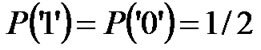 .
.
A popular approach in both simulation and commercial BERT test-sets is the assumption of PDF of “1” and “0” following Gaussian/normal distributions, i.e noise sources are approximated by Gaussian distributions. If the assumption is valid, high accuracy is achieved. This method enables a fast estimation of the BER by using the complementary error functions [25]:
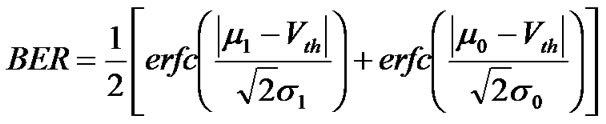 (31)
(31)
where  and
and  are the mean values for PDF of “1” and “0” respectively whereas
  and
and  are the variance of the PDFs. The quality factor - Q-factor which can be either in linear scale or in logarithmic scale can be calculated from the obtained BER through the expression:
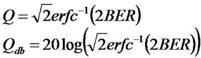 (32)
(32)
8.2.1. Improving Accuracy of Histogram
The common objective is to search for the proper values for number of bins and bin-width to be used in the approximation of the histogram so that the bias and the variance of the estimator can be negligible. According to [26], with a sufficiently large number of transmitted bits (N0), a good estimate for the width (Wbin) of each equally spaced histogram bin is given by: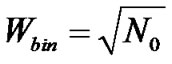 .
.
8.3. Optical Signal-to-Noise Ratio (OSNR)
The optical signal-to-noise ratio (OSNR) is a popular benchmark indicator for assessment of the performance of optical transmission systems, especially those limited by the ASE noise from the optical amplifiers – EDFAs. The OSNR is defined as the ratio of optical signal power to optical noise power. For a single EDFA with output power, Pout, the OSNR is given by:
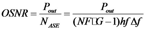 (33)
(33)
where NF is the amplifier noise figure, G is the amplifier gain, hf is the photon energy,  is the optical measurement bandwidth.
However, OSNR does not provide good estimation to the system performance when the main degrading sources involve the dynamic propagation effects such as dispersion (including both CD and PMD) and Kerr nonlinearity effects (eg. SPM). In these cases, the degradation of the performance is mainly due to waveform distortions rather than the corruption of the ASE or electronic noise. When addressing a value of an OSNR, it is important to define the optical measurement bandwidth over which the OSNR is calculated. The signal power and noise power is obtained by integrating all the frequency components across the bandwidth leading to the value of OSNR. In practice, signal and noise power values are usually measured directly from the optical spectrum analyzer (OSA), which does the mathematics for the users and displays the resultant OSNR versus wavelength or frequency over a fixed resolution bandwidth. A value of  = 0.1 nm or
  =12.5GHz is widely used as the typical value for calculation of the OSNR.
OSNR penalty is determined at a particular BER when varying value of a system parameter under test. For example, OSNR penalty at BER=1e-4 for a particular optical phase modulation format when varying length of an optical link in a long-haul transmission system configuration.
8.4. Eye Opening Penalty (EOP)
The OSNR is a time-averaged indicator for the system performance where the ratio of average power of optical carriers to noise is considered. When optical lightwaves

Figure 11. Demonstration of multi-peak/non-Gaussian distribution of the received electrical signal.
propagate through a dispersive and nonlinear optical fiber channel, the fiber impairments including ISI induced from CD, PMD and the spectral effects induced from nonlinearities cause the distortion of the waveforms. Another dynamic cause of the waveform distortion comes from the ISI effects as the results of optical or electrical filtering. In a conventional OOK system, bandwidth of an optical filter is normally larger than the spectral width of the signal by several times.
The eye-opening penalty (EOP) is a performance measure defined as the penalty of the “eye” caused by the distortion of the electrically detected waveforms to a reference eye-opening (EO). EO is the difference between the amplitudes of the lowest mark and the highest space.
The benchmark eye opening is usually obtained from a back-to-back measurement when the waveform is not distorted at all by any above impairments. The eye opening penalty at a particular sampling instance is normally calculated in log scale (dB unit) and given by:
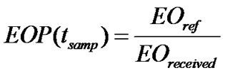 (34)
(34)
The EOP is useful for noise-free system evaluations as a good estimate of deterministic pulse distortion effects. The accuracy of EOP indicator depends on the sampling instance in a bit slot. Usually, the detected pulses are sampled at the instance giving the maximum eye opening. If noise is present, the calculation of the EOP become less precise because of the ambiguity of the signal levels which are corrupted by noise.
9. MATLAB Statistical Evaluation Techniques
The method using a Gaussian-based single distribution involves only the effects of noise corruption on the detected signals and ignores the dynamic distortion effects such as ISI and non-linearity. These dynamic distortions result in a multi-peak pdf as demonstrated in Figure 11, which is clearly overlooked by the conventional single distribution technique. As the result, the pdf of the electrical signal can not be approximated accurately. The addressed issues are resolved with the proposal of two new statistical methods.
Two new techniques proposed to accurately obtain the pdf of the detected electrical signal in optical communications include the mixture of multi-Gaussian distributions (MGD) by implementing the expectation maximization theory (EM) and the generalized Pareto distribution (GPD) of the generalized extreme values (GEV) theorem. These two techniques are well-known in fields of statistics, banking, finance, meteorology, etc. The implementation of required algorithms is carried out with MATLAB functions. Thus, these novel statistical methods offer a great deal of flexibility, convenience, fast-processing while maintaining the errors in obtaining the BER within small and acceptable limits.
9.1. Multi-Gaussian Distributions (MGD) via Expectation Maximization (EM)Theorem
The mixture density parameter estimation problem is probably one of the most widely used applications of the expectation maximization (EM) algorithm. It comes from the fact that most of deterministic distributions can be seen as the result of superposition of different multi distributions. Given a probability distribution function  for a set of received data,
  can be expressed as the mixture of M different distributions:
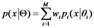 (35)
(35)
where the parameter are  such that
 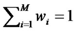 and each
  is a PDF by
  and each pdf having a weight
 , i.e probability of that PDF.
As a particular case adopted for optical communications, the EM algorithm is implemented with a mixture of multi Gaussian distributions (MGD). This method offers great potential solutions for evaluation of performance of an optical transmission system with following reasons: 1) In a linear optical system (low input power into fiber), the conventional single Gaussian distribution fails to take into account the waveform distortion caused by either the ISI due to fiber CD and PMD dispersion, the patterning effects. Hence, the obtained BER is no longer accurate. These issues however are overcome by using the MGD method. 2) Computational time for implementing MGD is fast via the EM algorithm which has become quite popular.
The selection of Number of Gaussian distributions for MGD Fitting can be conducted as follows. The critical step affecting the accuracy of the BER calculation is the process of estimate of the number of Gaussian distributions applied in the EM algorithm for fitting the received signal pdf. This number is determined by the estimated number of peaks or valleys in the curves of 1st and 2nd derivative of the original data set. Explanation of this procedure is carried out via the well-known “Hemming Lake Pike” example as reported in [27,28]. In this problem, the data of five age-groups give the lengths of 523 pike (Esox lucius), sampled in 1965 from Hemming Lake, Manitoba, Canada. The components are heavily overlapped and the resultant pdf is obtained with a mixture of these 5 Gaussian distributions as shown in Figure 12(a). The figures are extracted from [29] for demonstration of the procedure.
Figure 12. Five contributed Gaussian distributions.
Estimation of number of Gaussian distributions in the mixed pdf based on 1st and 2nd derivatives of the original data set (courtesy from [29]). As seen from Figure 12, the 1st derivative of the resultant pdf shows clearly 4 pairs of peaks (red) and valleys (blue), suggesting that there should be at least 4 component Gaussian distributions contributing to the original pdf. However, by taking the 2nd derivative, it is realized that there is actually up to 5 contributed Gaussian distributions as shown in Figure 12.
In summary, the steps for implementing the MGD technique to obtain the BER value is described in short as follows: 1) Obtaining the pdf from the normalized histogram of the received electrical levels; 2) Estimating the number of Gaussian distributions (NGaus) to be used for fitting the pdf of the original data set; 3) Applying EM algorithm with the mixture of NGaus Gaussian distributions and obtaining the values of mean, variance and weight for each distribution; 4) Calculating the BER value based on the integrals of the overlaps of the Gaussian distributions when the tails of these distributions cross the threshold.
9.2. Generalized Pareto Distribution (GPD)
The GEV theorem is used to estimate the distribution of a set of data of a function in which the possibility of extreme data lengthen the tail of the distribution. Due to the mechanism of estimation for the pdf of the extreme data set, GEV distributions can be classified into two classes consisting of the GEV distribution and the generalized Pareto distribution (GPD).
There has recently been only a countable number of research studies on the application of this theorem into optical communications. However, these studies only reports on the GEV distributions which only involves the effects of noise and neglect the effects of dynamic distortion factors.
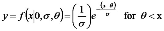
Unlike the Gaussian-based techniques but rather similar to the exponential distribution, the generalized Pareto distribution is used to model the tails of distribution. This section provides an overview of the generalized Pareto distribution (GPD). The probability density function for the generalized Pareto distribution is defined as follows:
 (36)
(36)

where k is shape parameter k ≠ 0, σ is scale parameter and the threshold parameter θ.
Equation (36) has significant constraints given as
•When k>0:  i.e there is no upper bound for x
• When k<0:  and zero probability for the case
•When k = 0, i.e Equation turning to:
•If k = 0 and θ = 0, the generalized Pareto distribution is equivalent to the exponential distribution.
•If k > 0 and θ = σ, the generalized Pareto distribution is equivalent to the Pareto distribution.
The GPD has three basic forms reflecting different class of underlying distributions.
•Distributions whose tails decrease exponentially, such as the normal distribution, lead to a generalized Pareto shape parameter of zero.
•Distributions with tails decreasing as a polynomial, such as Student’s t lead to a positive shape parameter.
• Distributions having finite tails, such as the beta, lead to a negative shape parameter.
GPD is widely used in fields of finance, meteorology, material engineering, etc… to for the prediction of extreme or rare events which are normally known as the exceedances. However, GPD has not yet been applied in optical communications to obtain the BER. The following reasons suggest that GPD may become a potential and a quick method for evaluation of an optical system, especially when non-linearity is the dominant degrading factor to the system performance.
1) The normal distribution has a fast roll-off, i.e. short tail. Thus, it is not a good fit to a set of data involving exeedances, i.e. rarely happening data located in the tails of the distribution. With a certain threshold value, the generalized Pareto distribution can be used to provide a good fit to extremes of this complicated data set.
2) When nonlinearity is the dominating impairment degrading the performance of an optical system, the sampled received signals usually introduce a long tail distribution. For example, in case of DPSK optical system, the distribution of nonlinearity phase noise differs from the Gaussian counterpart due to its slow roll-off of the tail. As the result the conventional BER obtained from assumption of Gaussian-based noise is no longer valid and it often underestimates the BER.
3) A wide range of analytical techniques have recently been studied and suggested such as importance sampling, multi-canonical method, etc. Although these techniques provide solutions to obtain a precise BER, they are usually far complicated. Whereas, calculation of GPD has become a standard and available in the recent Matlab version (since Matlab 7.1). GPD therefore may provide a very quick and convenient solution for monitoring and evaluating the system performance. Necessary preliminary steps which are fast in implementation need to be carried out the find the proper threshold.
4) Evaluation of contemporary optical systems requires BER as low as 1e-15. Therefore, GPD can be seen quite suitable for optical communications.
9.2.1. Selection of Threshold for GPD Fitting
Using this statistical method, the accuracy of the obtained BER strongly depend on the threshold value (Vthres) used in the GPD fitting algorithm, i.e. the decision where the tail of the GPD curve starts.
There have been several suggested techniques as the guidelines aiding the decision of the threshold value for the GPD fitting. However, they are not absolute techniques and are quite complicated. In this paper, a simple technique to determine the threshold value is proposed. The technique is based on the observation that the GPD tail with exceedances normally obeying a slow exponential distribution compared to the faster decaying slope of the distribution close to the peak values. The inflection region between these two slopes gives a good estimation of the threshold value for GPD fitting. This is demonstrated in Figure 13.
Whether the selection of the Vthres value leads to an adequately accurate BER or not is evaluated by using the cumulative density function (cdf-Figure 14) and the quantile-quantile plot (QQ plot Figure 15). If there is a high correlation between the pdf of the tail of the original data set (with a particular Vthres) and pdf of the GPD, there would be a good fit between empirical cdf of the data set with the GPD-estimated cdf with focus at the most right region of the two curves. In the case of the QQ-plot, a linear trend would be observed. These guidelines are illustrated in Figure 14. In this particular case, the value of 0.163 is selected to be Vthres.
Furthermore, as a demonstration of improper selection of Vthres, the value of 0.2 is selected. Figure 16 and Figure 17 show the non-compliance of the fitted curve with the GPD which is reflected via the discrepancy in the two cdfs and the nonlinear trend of the QQ-plot.
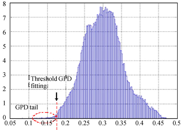
Figure 13. Selection of threshold for GPD fitting.
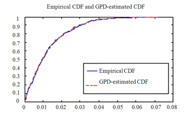
Figure 14. Comparison between fitted and empirical cumulative distribution functions.

Figure 15. Quantile-quantile plot.
Figure 16. Comparison between fitted and empirical cumulative distribution functions.
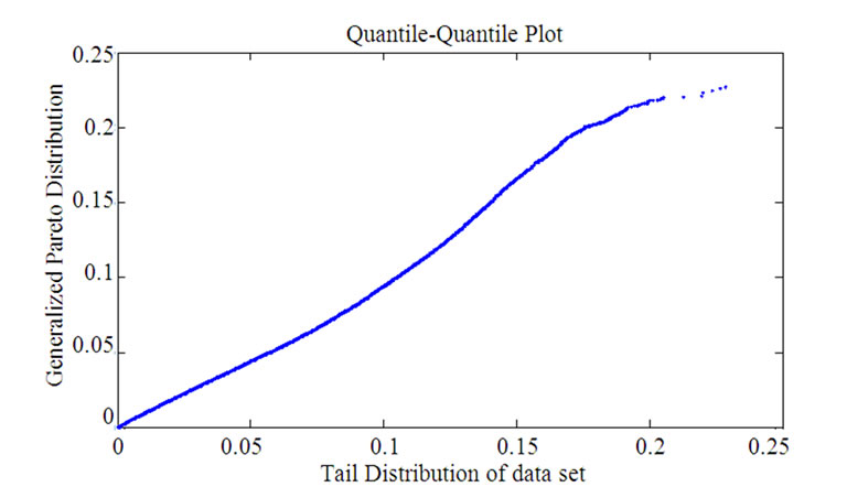
Figure 17. Quantile-quantile plot.
9.3. Validation of the Statistical Methods
A simulation test-bed of an optical DPSK transmission system over 880 km SSMF dispersion managed optical link (8 spans) is set up. Each span consists of 100 km SSMF and 10 km of DCF whose dispersion values are +17 ps/nm.km and -170 ps/nm.km at 1550 nm wavelength respectively and fully compensated i.e zero residual dispersion. The average optical input power into each span is set to be higher than the nonlinear threshold of the optical fiber. The degradation of the system performance hence is dominated by the nonlinear effects which are of much interest since it is a random process creating indeterminate errors in the long tail region of the pdf of the received electrical signals.
The BER results obtained from the novel statistical methods are compared to that from the Monte-Carlo simulation as well as from the semi-analytical method. Here, the well-known analytical expression to obtain the BER of the optical DPSK format is used, given as [30].
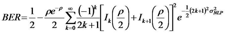 (37)
(37)
where  is the obtained OSNR and
  is the variance of nonlinear phase noise.
In this case, in order to calculate the BER of a optical DPSK system involving the effect of nonlinear phase noise, the required parameters including the OSNR and the variance of nonlinear phase noise etc are obtained from the simulation numerical data which is stored and processed in Matlab. The fitting curves implemented with the MGD method for the pdf of bit 0 and bit 1 (input power of 10 dBm) as shown in Figure 18 and illustrated in Figure 19 for bit 0 and bit 1 respectively.
The selection of optimal threshold for GPD fitting follows the guideline as addressed in detail in the previous section. The BER from various evaluation methods are shown in Table 1. The input powers are controlled to be 10 dBm and 11 dBm.
Table 1 validates the adequate accuracy of the proposed novel statistical methods with the discrepancies compared to the Monte-Carlo and semi-analytical BER to be within one decade. In short, these methods offer a great deal of fast processing while maintaining the accuracy of the obtained BER within the acceptable limits.
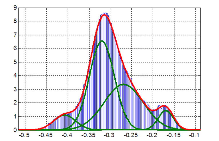
Figure 18. Demonstration of fitting curves for bit ‘0’ with MGD method.
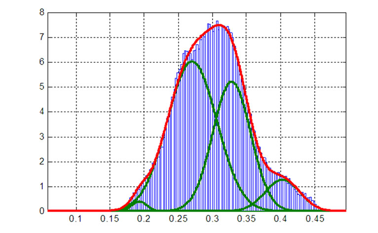
Figure 19. Demonstration of fitting curves for bit ‘0’ with MGD method.
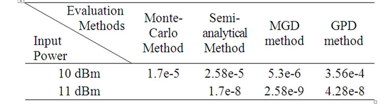
Table 1. The BER from various evaluation methods.
10. Conclusions
We have demonstrated the Simulink modeling of amplitude and phase modulation formats at 40 Gb/s optical fiber transmission. A novel modified fiber propagation algorithm has been used to minimize the simulation processing time and optimize its accuracy. The principles of amplitude and phase modulation, encoding and photonic-opto-electronic balanced detection and receiving modules have been demonstrated via Simulink modules and can be corroborated with experimental receiver sensitivities.
The XPM and other fiber nonlinearity such as the Raman scattering, four wave mixing are not integrated in the Matlab Simulink models. A switching scheme between the linear only and the linear and nonlinear models is developed to enhance the computing aspects of the transmission model.
Other modulations formats such as multi-level MDPSK, M-ASK that offer narrower effective bandwidth, simple optical receiver structures and no chirping effects would also be integrated. These systems will be reported in future works. The effects of the optical filtering components in DWDM transmission systems to demonstrate the effectiveness of the DPSK and DQPSK formats, have been measured in this paper and will be verified with simulation results in future publications. Finally, further development stages of the simulator together with simulation results will be reported in future works.
We have illustrated the modeling of various schemes of advanced modulation formats for optical transmission systems. Transmitter modules integrating lightwaves sources, electrical pre-coder and external modulators can be modeled without difficulty under MATLAB Simulink. As the popularity of MATLAB becoming a standard computing language for academic research institutions throughout the world, the models reported here would contribute to the wealth of computing tools for modeling optical fiber transmission systems and teaching undergraduates at senior level and postgraduate research scholars. The models can integrate photonic filters or other photonic components using blocksets available in Simulink. Furthermore we have used the developed models to assess the effectiveness of the models by evaluating the simulated results and experimental transmission performance of long haul advanced modulation format transmission systems.
11. References
[1] L. N. Binh, “Tutorial Part I on optical systems design,” ECE 4405, ECSE Monash University, Australia, presented at ICOCN 2002.
[2] T. Kawanishi, S. Shinada, T. Sakamoto, S. Oikawa, K. Yoshiara, and M. Izutsu, “Reciprocating optical modulator with resonant modulating electrode,” Electronics Letters, Vol. 41, No. 5, pp. 271-272, 2005.
[3] R. Krahenbuhl, J. H. Cole, R. P. Moeller, and M. M. Howerton, “High-speed optical modulator in LiNbO3 with cascaded resonant-type electrodes,” Journal of Lightwave Technology, Vol. 24, No. 5, pp. 2184-2189, 2006.
[4] I. P. Kaminow and T. Li, “Optical fiber communications,” Vol. IVA, Elsevier Science, Chapter 16, 2002.
[5] G. P. Agrawal, “Fiber-optic communications systems,” 3rd edition, John Wiley & Sons, 2001.
[6] J. B. Jeunhomme, “Single mode fiber optics,” Principles and Applications, 2nd edition: Marcel Dekker Pub, 1990.
[7] E. E. Basch, (Editor in Chief), “Optical-fiber transmission,” 1st edition, SAMS, 1987.
[8] I. P. Kaminow and T. Li, “Optical fiber communications,” Vol. IVB, Elsevier Science (USA), Chapter 5, 2002.
[9] J. P. Gordon and H. Kogelnik, “PMD fundamentals: Polarization mode dispersion in optical fibers,” PNAS, Vol. 97, No. 9, pp. 4541-4550, April 2000.
[10] Corning. Inc, “An introduction to the fundamentals of PMD in fibers,” White Paper, July 2006.
[11] A. Galtarossa and L. Palmieri, “Relationship between pulse broadening due to polarisation mode dispersion and differential group delay in long singlemode fiber,” Electronics Letters, Vol. 34, No. 5, March 1998.
[12] J. M. Fini and H. A. Haus, “Accumulation of polarization-mode dispersion in cascades of compensated optical fibers,” IEEE Photonics Technology Letters, Vol. 13, No. 2, pp. 124-126, February 2001.
[13] A. Carena, V. Curri, R. Gaudino, P. Poggiolini, and S. Benedetto, “A time-domain optical transmission system simulation package accounting for nonlinear and polarization-related effects in fiber,” IEEE Journal on Selected Areas in Communications, Vol. 15, No. 4, pp. 751-765, 1997.
[14] S. A. Jacobs, J. J. Refi, and R. E. Fangmann, “Statistical estimation of PMD coefficients for system design,” Electronics Letters, Vol. 33, No. 7, pp. 619-621, March 1997.
[15] E. A. Elbers, International Journal Electronics and Communications (AEU) 55, pp 195-304, 2001.
[16] T. Mizuochi, K. Ishida, T. Kobayashi, J. Abe, K. Kinjo, K. Motoshima, and K. Kasahara, “A comparative study of DPSK and OOK WDM transmission over transoceanic distances and their performance degradations due to nonlinear phase noise,” Journal of Lightwave Technology, Vol. 21, No. 9, pp. 1933-1943, 2003.
[17] H. Kim, “Differential phase shift keying for 10-Gb/s and 40-Gb/s systems,” in Proceedings of Advanced Modulation Formats, 2004 IEEE/LEOS Workshop on, pp. 13-14, 2004.
[18] P. J. T. Tokle., “Advanced modulation fortmas in 40 Gbit/s optical communication systems with 80 km fiber spans,” Elsevier Science, July 2003.
[19] Elbers, et al., International Journal of Electronics Communications (AEU) 55, pp 195-304, 2001.
[20] J. P. Gordon and L. F. Mollenauer, “Phase noise in photonic communications systems using linear amplifiers,” Optics Letters, Vol. 15, No. 23, pp. 1351-1353, December 1990.
[21] G. Jacobsen, “Performance of DPSK and CPFSK systems with significant post-detection filtering,” IEEE Journal of Lightwave Technology, Vol. 11, No. 10, pp. 1622-1631, 1993.
[22] A. F. Elrefaie and R. E. Wagner, “Chromatic dispersion limitations for FSK and DPSK systems with direct detec tion receivers,” IEEE Photonics Technology Letters, Vol. 3, No. 1, pp. 71-73, 1991.
[23] A. F. Elrefaie, R. E. Wagner, D. A. Atlas, and A. D. Daut, “Chromatic dispersion limitation in coherent lightwave systems”, IEEE Journal of Lightwave Technology, Vol. 6, No. 5, pp. 704-710, 1988.
[24] D. E. Johnson, J. R. Johnson, and a. H. P. Moore, “A handbook of active filters,” Englewood Cliffs, New Jersey: Prentice-Hall, 1980.
[25] J. G. Proakis, “Digital communications,” 4th edition, New York: McGraw-Hill, 2001.
[26] W. H. Tranter, K. S. Shanmugan, T. S. Rappaport, and K. L. Kosbar, “Principles of communication systems simulation with wireless applications,” New Jersey: Prentice Hall, 2004.
[27] P. D. M. Macdonald, “Analysis of length-frequency distributions,” in Age and Growth of Fish,. Ames Iowa: Iowa State University Press, pp. 371-384, 1987.
[28] P. D. M. Macdonald and T. J. Pitcher, “Age-groups from size-frequency data: A versatile and efficient method of analyzing distribution mixtures,” Journal of the Fisheries Research Board of Canada, Vol. 36, pp. 987-1001, 1979.
[29] E. F. Glynn, “Mixtures of Gaussians,” Stowers Institute for Medical Research, February 2007, http://research. stowers-institute.org/efg/R/Statistics/MixturesOfDistributions/index.htm.
[30] K. P. Ho, “Performance degradation of phase-modulated systems due to nonlinear phase noise,” IEEE Photonics Technology Letters, Vol. 15, No. 9, pp. 1213-1215, 2003.
Appendix: A Matlab program of the split-step propagation of the guided lightwave signals
function output = ssprop_matlabfunction_raman(input)
nt = input(1);
u0 = input(2:nt+1);
dt = input(nt+2);
dz = input(nt+3);
nz = input(nt+4);
alpha_indB = input(nt+5);
betap = input(nt+6:nt+9);
gamma = input(nt+10);
P_non_thres = input(nt+11);
maxiter = input(nt+12);
tol = input(nt+13);
%Ld = input(nt+14);
%Aeff = input(nt+15);
%Leff = input(nt+16);
tic;
%tmp = cputime;
%----------------------------------------------------------
%----------------------------------------------------------
% This function ssolves the nonlinear Schrodinger equation for % pulse propagation in an optical fiber using the split-step % Fourier method % % The following effects are included in the model: group velocity % dispersion (GVD), higher order dispersion, loss, and self-phase % modulation (gamma).
% % USAGE % % u1 = ssprop(u0,dt,dz,nz,alpha,betap,gamma);
% u1 = ssprop(u0,dt,dz,nz,alpha,betap,gamma,maxiter);
% u1 = ssprop(u0,dt,dz,nz,alpha,betap,gamma,maxiter,tol);
% % INPUT % % u0 - starting field amplitude (vector)
% dt - time step - [in ps]
% dz - propagation stepsize - [in km]
% nz - number of steps to take, ie, ztotal = dz*nz % alpha - power loss coefficient [in dB/km], need to convert to linear to have P=P0*exp(-alpha*z)
% betap - dispersion polynomial coefs, [beta_0 ... beta_m] [in ps^(m-1)/km]
% gamma - nonlinearity coefficient [in (km^-1.W^-1)]
% maxiter - max number of iterations (default = 4)
% tol - convergence tolerance (default = 1e-5)
% % OUTPUT % % u1 - field at the output
%--------------
% Convert alpha_indB to alpha in linear domain
%-------------
-alpha = 1e-3*log(10)*alpha_indB/10;
% alpha (1/km) - see Agrawal p57
%--------------%
P_non_thres = 0.0000005;
ntt = length(u0);
w = 2*pi*[(0:ntt/2-1),(-ntt/2:-1)]'/(dt*nt);
%t = ((1:nt)'-(nt+1)/2)*dt;
gain = numerical_gain_hybrid(dz,nz);
for array_counter = 2:nz+1
grad_gain(1) = gain(1)/dz;
grad_gain(array_counter) = (gain(array_counter)-gain(array_counter-1))/dz;
end gain_lin = log(10)*grad_gain/(10*2);
clear halfstep
halfstep = -alpha/2;
for ii = 0:length(betap)-1;
halfstep = halfstep - j*betap(ii+1)*(w.^ii)/factorial(ii);
end
square_mat = repmat(halfstep, 1, nz+1);
square_mat2 = repmat(gain_lin, ntt, 1);
size(square_mat);
size(square_mat2);
total = square_mat + square_mat2;
clear LinearOperator
% Linear Operator in Split Step method
LinearOperator = halfstep;
halfstep = exp(total*dz/2);
u1 = u0;
ufft = fft(u0);
% Nonlinear operator will be added if the peak power is greater than the % Nonlinear threshold iz = 0;
while (iz < nz) && (max((gamma*abs(u1).^2 + gamma*abs(u0).^2)) > P_non_thres)
iz = iz+1;
uhalf = ifft(halfstep(:,iz).*ufft);
for ii = 1:maxiter uv = uhalf .* exp((-j*(gamma)*abs(u1).^2 + (gamma)*abs(u0).^2)*dz/2);
ufft = halfstep(:,iz).*fft(uv);
uv = ifft(ufft);
if (max(uv-u1)/max(u1) < tol)
u1 = uv;
break;
else
u1 = uv;
end
end
% fprintf('You are using SSFM\n');
if (ii == maxiter)
fprintf('Failed to converge to %f in %d iterations',tol,maxiter);
end
u0 = u1;
end if (iz < nz) && (max((gamma*abs(u1).^2 + gamma*abs(u0).^2)) < P_non_thres)
% u1 = u1.*rectwin(ntt);
ufft = fft(u1);
ufft = ufft.*exp(LinearOperator*(nz-iz)*dz);
u1 = ifft(ufft);
%fprintf('Implementing Linear Transfer Function of the Fibre Propagation');
end
NOTES
1http://www.mathworks.com/, access date: August 22, 2008.