Journal of Water Resource and Protection, 2013, 5, 377-394
http://dx.doi.org/10.4236/jwarp.2013.54038 Published Online April 2013 (http://www.scirp.org/journal/jwarp)
Laboratory Validation of an Integrated Surface Water—
Groundwater Model
T. D. Sparks, B. N. Bockelmann-Evans, R. A. Falconer
Hydro-Environmental Research Centre, Cardiff School of Engineering, Cardiff University, Cardiff, UK
Received November 29, 2012; revised January 5, 2013; accepted January 20, 2013
Copyright © 2013 T. D. Sparks, et al. This is an open access article distributed under the Creative Commons Attribution License,
which permits unrestricted use, distribution, and reproduction in any medium, provided the original work is properly cited.
ABSTRACT
The hydrodynamic surface water model DIVAST has been extended to include horizontally adjacent groundwater flows.
This extended model is known as DIVAST-SG (Depth Integrated Velocities and Solute Transport with Surface Water
and Groundwater). After development and analytical verification the model was tested against a novel laboratory set-up
using open cell foam (60 pores per inch—ppi) as an idealised porous media representing a riverbank. The Hyder Hy-
draulics Laboratory at Cardiff University has a large tidal basin that was adapted to simulate a surface water—ground-
water scenario using this foam, and used to validate the DIVAST-SG model. The properties of the laboratory set-up
were measured and values were determined for hydraulic conductivity (permeability) and porosity, evaluated as 0.002
m/s and 75% respectively. Lessons learnt in this initial experimentation were used to modify the flume construction and
improve the experimental procedure, with further experimentation being undertaken of both water level variations and
tracer movement. Valuable data have been obtained from the laboratory experiments, allowing the validity of the nu-
merical model to be assessed. Modifications to the input file to include representations of the joints between the foam
blocks allowed a good fit between the observed and modelled water levels. Encouraging correlation was observed in
tracer experiments using Rhodamine-WT dye between the observed exit points of the tracer from the foam, and the
modelled exit points with time.
Keywords: Integrated Surface Water Groundwater Modelling; Laboratory Experiments; Open Cell Foam
1. Introduction
Surface water and groundwater—two different resources
—require careful management and protection. Computer
modelling of both resources has long been used as an aid
to the management of water resources. Historically,
groundwater and surface water flows have been modelled
separately, as their behaviour is represented by different
mathematical equations and over very different time
scales. However, these flow processes are a linked re-
source; one depends upon and impacts on the other.
Groundwater provides a third of the United Kingdom’s
drinking water, and in some areas of southern England
up to 80% of the drinking water comes from groundwater
resources. Usually it requires little or no treatment before
it is drinkable. However, if contaminated, these resources
are expensive and difficult to restore, so groundwater
needs to be protected. Surface water in rivers, lakes, es-
tuaries and coastal systems is more visibly abundant, but
no less important—its behaviour affects our everyday
lives through flooding, leisure activities, transport, drink-
ing water etc. These two resources are integral; the base-
flow in streams and rivers comes from the contributing
groundwater; agricultural chemicals may seep into ground-
water, which subsequently may flow into streams. Accu-
rate modelling of surface water flows needs to include
contributions from groundwater resources, which can
contribute significantly to the behaviour of free surface
flows.
Historically, both open channel and groundwater flows
have been considered for solution by numerical methods.
Where the two “zones” meet, the problem has usually
been approached by calculating the response of the
groundwater system to changes in the river elevation
[1,2]. [3] developed a model describing infiltration and
overland flow based on the soil moisture properties. [4]
took this approach a stage further and described numeri-
cal solutions to the coupled boundary problems repre-
senting 3-D, transient, saturated-unsaturated subsurface
flow, and 1-D, gradually varied, unsteady channel flow.
C
opyright © 2013 SciRes. JWARP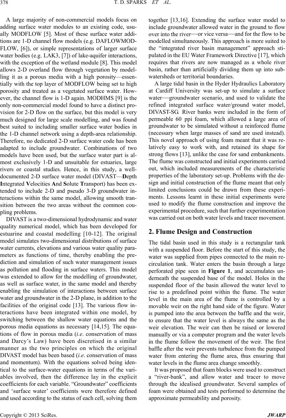

T. D. SPARKS ET AL. 378
A large majority of non-commercial models focus on
adding surface water modules to an existing code, usu-
ally MODFLOW [5]. Most of these surface water addi-
tions are 1-D channel flow models (e.g. DAFLOWMOD-
FLOW, [6]), or simple representations of larger surface
water bodies (e.g. LAK3, [7]) of lake-aquifer interactions,
with the exception of the wetland module [8]. This model
allows 2-D overland flow through vegetation by model-
ling it as a porous media with a high porosity—essen-
tially with the top layer of MODFLOW being set to high
porosity and treated as a vegetated surface water. How-
ever, the channel flow is 1-D again. MODHMS [9] is the
only non-commercial model found to have a distinct pro-
vision for 2-D flow on the surface, but this model is very
much designed for large scale modelling, and was found
best suited to including smaller surface water bodies in
the 1-D channel network using a depth-area relationship.
Therefore, no dedicated 2-D surface water code has been
adapted to include groundwater. Combinations of two
models have been used, but the surface water part is al-
most exclusively 1-D and unsuitable for estuaries, large
rivers or coastal studies. Hence, in this study, a well-
documented 2-D surface water model (DIVAST—Depth
Integrated Velocities And Solute Transport) has been ex-
tended to include 2-D and pseudo 3-D groundwater in-
teractions within the same model, allowing smooth tran-
sition between the two areas without the common cou-
pling problems.
DIVAST is a two-dimensional hydrodynamic and water
quality numerical model, which has been developed for
estuarine and coastal modelling [10-12]. The original
model simulates two-dimensional distributions of surface
water currents, elevations and various water quality para-
meters as functions of time, thereby enabling the pre-
diction and simulation of such water management issues
as pollution and flooding in surface waters. This model
was extended to allow for the modelling of groundwater,
as well as surface water, in the same model and thereby
enabling the simulation of interactions between surface
water and groundwater in the 2-D plane, in addition to the
facilities of the original code [13]. The various flow in-
teractions have been integrated within one model, by
switching between the shallow water equations and the
porous media equations as necessary [14,15]. The equa-
tions of flow in porous media (i.e. conservation of mass
and Darcy’s Law) have been discretised in a similar
manner as the two principles on which the original
DIVAST model has been based (i.e. conservation of mass
and momentum). With the equations solved being iden-
tical to the surface-water equations in terms of the vari-
ables involved, then the difference lay in the explicit
coefficients for each variable. “Groundwater” coefficients
and ‘surface water’ coefficients were therefore defined
and used according to the status of each cell, solving them
together [13,16]. Extending the surface water model to
include groundwater allowed water in the ground to flow
over into the river—or vice versa—and for the flow to be
modelled simultaneously. This approach is more suited to
the “integrated river basin management” approach sti-
pulated in the EU Water Framework Directive [17], which
requires that rivers are now managed as a whole river
basin, rather than artificially dividing them up into sub-
watersheds or territorial boundaries.
A large tidal basin in the Hyder Hydraulics Laboratory
at Cardiff University was set-up to simulate a surface
water—groundwater scenario, and used to validate the
refined integrated surface water/ground water model,
DIVAST-SG. River banks were included in the form of
permeable 60 ppi foam, which allowed a large area of
groundwater to be simulated without a reinforced flume
(necessary when large masses of sand are used instead).
This novel approach of using foam meant that it was re-
latively easy to work with, and retained its shape for
strong flows [13], unlike the case for sand embankments.
The flume was constructed and initial experiments carried
out, which included measurements of the characteristic
properties of the laboratory set-up. Problems with the de-
sign and initial construction of the flume meant that only
limited conclusions could be drawn from these experi-
ments. Lessons learnt in these initial experiments were
used to modify the flume construction and improve the
experimental procedure, such that further experimentation
was carried out on both water levels and tracer movement.
2. Flume Design and Construction
The tidal basin used in this study is a rectangular tank
with a suspended floor. Before the start of this study, the
water was supplied from pipes connected to the main re-
circulation tank. Water enters the basin through a large
perforated pipe seen in Figure 1, and accumulates un-
derneath the suspended base of the model. Holes in the
suspended floor of the basin allowed the water level to
rise to a predefined point within the flume. The water
level in the main area of the flume is controlled by a
movable weir on the right hand side of the figure. Water
is pumped into the area between the baffle and the weir,
to ensure that the water level is always the same as the
weir elevation. The weir can then be raised or lowered
manually or via a computer program and the water levels
in the flume follow the movement of the weir. The first
baffle after the weir prevents turbulence from the pumped
water from entering the flume area, thus ensuring that
water levels in the flume area change smoothly.
It was proposed that foam blocks were used to construct
a “river-bank”, and allow water and tracer to move
through the idealised groundwater. Several samples of
foam were obtained and tests performed to determine the
approximate permeability and porosity.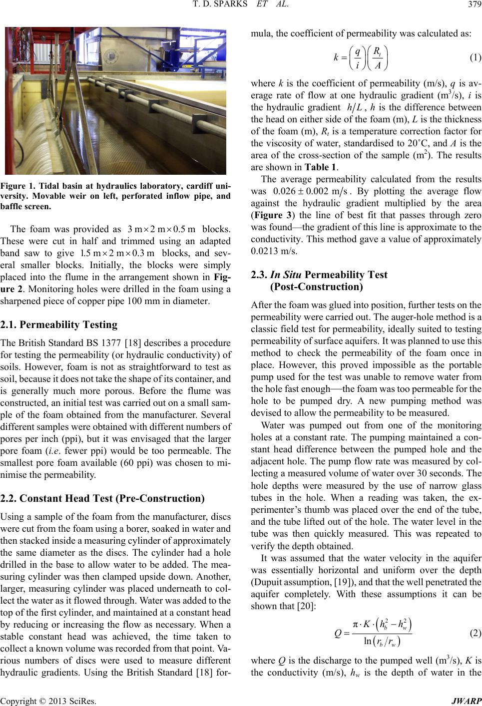

T. D. SPARKS ET AL. 379
Figure 1. Tidal basin at hydraulics laboratory, cardiff uni-
versity. Movable weir on left, perforated inflow pipe, and
baffle screen.
The foam was provided as blocks.
These were cut in half and trimmed using an adapted
band saw to give 1. blocks, and sev-
eral smaller blocks. Initially, the blocks were simply
placed into the flume in the arrangement shown in Fig-
ure 2. Monitoring holes were drilled in the foam using a
sharpened piece of copper pipe 100 mm in diameter.
3m
5 m2 m0.3
2m 0.5m
m
2.1. Permeability Testing
The British Standard BS 1377 [18] describes a procedure
for testing the permeability (or hydraulic conductivity) of
soils. However, foam is not as straightforward to test as
soil, because it does not take the shape of its container, and
is generally much more porous. Before the flume was
constructed, an initial test was carried out on a small sam-
ple of the foam obtained from the manufacturer. Several
different samples were obtained with different numbers of
pores per inch (ppi), but it was envisaged that the larger
pore foam (i.e. fewer ppi) would be too permeable. The
smallest pore foam available (60 ppi) was chosen to mi-
nimise the permeability.
2.2. Constant Head Test (Pre-Construction)
Using a sample of the foam from the manufacturer, discs
were cut from the foam using a borer, soaked in water and
then stacked inside a measuring cylinder of approximately
the same diameter as the discs. The cylinder had a hole
drilled in the base to allow water to be added. The mea-
suring cylinder was then clamped upside down. Another,
larger, measuring cylinder was placed underneath to col-
lect the water as it flowed through. Water was added to the
top of the first cylinder, and maintained at a constant head
by reducing or increasing the flow as necessary. When a
stable constant head was achieved, the time taken to
collect a known volume was recorded from that point. Va-
rious numbers of discs were used to measure different
hydraulic gradients. Using the British Standard [18] for-
mula, the coefficient of permeability was calculated as:
t
R q
kiA
 


 
(1)
where k is the coefficient of permeability (m/s), q is av-
erage rate of flow at one hydraulic gradient (m3/s), i is
the hydraulic gradient hL, h is the difference between
the head on either side of the foam (m), L is the thickness
of the foam (m), Rt is a temperature correction factor for
the viscosity of water, standardised to 20˚C, and A is the
area of the cross-section of the sample (m2). The results
are shown in Table 1.
The average permeability calculated from the results
was 0.0260.002 ms

. By plotting the average flow
against the hydraulic gradient multiplied by the area
(Figure 3) the line of best fit that passes through zero
was found—the gradient of this line is approximate to the
conductivity. This method gave a value of approximately
0.0213 m/s.
2.3. In Situ Permeability Test
(Post-Construction)
After the foam was glued into position, further tests on the
permeability were carried out. The auger-hole method is a
classic field test for permeability, ideally suited to testing
permeability of surface aquifers. It was planned to use this
method to check the permeability of the foam once in
place. However, this proved impossible as the portable
pump used for the test was unable to remove water from
the hole fast enough—the foam was too permeable for the
hole to be pumped dry. A new pumping method was
devised to allow the permeability to be measured.
Water was pumped out from one of the monitoring
holes at a constant rate. The pumping maintained a con-
stant head difference between the pumped hole and the
adjacent hole. The pump flow rate was measured by col-
lecting a measured volume of water over 30 seconds. The
hole depths were measured by the use of narrow glass
tubes in the hole. When a reading was taken, the ex-
perimenter’s thumb was placed over the end of the tube,
and the tube lifted out of the hole. The water level in the
tube was then quickly measured. This was repeated to
verify the depth obtained.
It was assumed that the water velocity in the aquifer
was essentially horizontal and uniform over the depth
(Dupuit assumption, [19]), and that the well penetrated the
aquifer completely. With these assumptions it can be
shown that [20]:



22
π
ln
bw
bw
K
hh
Qrr
 
 (2)
where Q is the discharge to the pumped well (m3/s), K is
the conductivity (m/s), hw is the depth of water in the

T. D. SPARKS ET AL.
Cops. JWARP
380
Figure 2. Layout of foam blocks in flume and initial set-up of channel.
Table 1. Summary of results and calculations.
No. of
discs H (head) (m) L (thickness) (m) Average flow (m3/s) dh/dL Cross section area
(m2) dh/dL *area K (m/s)
2 0.033 0.030 1.29E−05 1.111852 0.0005996 0.000667 1.93E−02
3 0.033 0.045 1.02E−05 0.741235 0.0005996 0.000444 2.31E−02
4 0.033 0.060 8.44E−06 0.555926 0.0005996 0.000333 2.53E−02
5 0.033 0.075 6.02E−06 0.444741 0.0005996 0.000267 2.26E−02
Average 2.26E−02
Standard deviation 2.16E−03
Calculating the Permeability of Foam.
3x
50.0006 0.000
flow (m
3
/s)
y = 0. 021
0.00E+00
2.00E-06
4.00E-06
6.00E-06
8.00E-06
1.00E-05
1.20E-05
1.40E-05
1.60E-05
00.00010.0002 0.0003 0.0004 0.0007

yright © 2013 SciRe
ex per iment al dat a
line of best fit (zero intercept)
K = 0.0213 m/ s

hydraulic gradient × area (m2)
Figure 3. Hydraulic gradient × area, against flow, enabling
the permeability to be calculated from the gradient of the
line.
aquifer at the pumped well

m, hb is the depth of water
at the boundary well (m), rw is the radius of pumped well
(m), rb is the radius of the circle from the centre of the
pumped well to the centre of the boundary well.
Rearranging Equation (2) in terms of K gives:
22
ln
π
b
w
bw
r
Qr
Khh



 (3)
This equation can be used to approximate the perme-
ability of the foam. The experimental results and calcu-
lated permeabilities are shown in Table 2.
This can be confirmed by an iterative method carried
out as follows. A linear head distribution between the two
wells was assumed to start with (with heads at the wells
being taken from the data collected above), and the
permeability was estimated at intervals between the two
wells, using Darcy’s Law (Equation (1)). If the estimate of
the head distribution is correct, each interval should give a
similar value for the conductivity. The initial linear head
distribution gave values for K which vary widely between
the wells, and so was obviously incorrect. The heads
across the area were then varied according to an arbitrary
equation based on
y
x, and iteration was halted when
the variation of the K values across the domain was at a
minimum.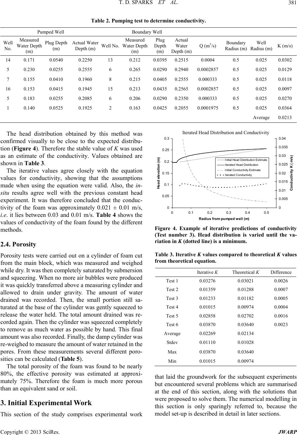

T. D. SPARKS ET AL. 381
Table 2. Pumping test to determine co nduc tivity.
Pumped Well Boundary Well
Well
No.
Measured
Water Depth
(m)
Plug Depth
(m)
Actual Water
Depth (m) Well No.
Measured
Water Depth
(m)
Plug
Depth
(m)
Actual
Water
Depth (m)
Q (m3/s) Boundary
Radius (m)
Well
Radius (m)K (m/s)
14 0.171 0.0540 0.2250 13 0.212 0.03950.25150.0004 0.5 0.025 0.0302
5 0.230 0.0255 0.2555 6 0.265 0.02900.29400.0002857 0.5 0.025 0.0129
7 0.155 0.0410 0.1960 8 0.215 0.04050.25550.000333 0.5 0.025 0.0118
16 0.153 0.0415 0.1945 15 0.213 0.04350.25650.00028570.5 0.025 0.0097
5 0.183 0.0255 0.2085 6 0.206 0.02900.23500.000333 0.5 0.025 0.0270
1 0.140 0.0525 0.1925 2 0.163 0.04250.20550.0001975 0.5 0.025 0.0364
Average0.0213
The head distribution obtained by this method was
confirmed visually to be close to the expected distribu-
tion (Figure 4). Therefore the stable value of K was used
as an estimate of the conductivity. Values obtained are
shown in Table 3.
The iterative values agree closely with the equation
values for conductivity, showing that the assumptions
made when using the equation were valid. Also, the in-
situ results agree well with the previous constant head
experiment. It was therefore concluded that the conduc-
tivity of the foam was approximately 0.021 ± 0.01 m/s,
i.e. it lies between 0.03 and 0.01 m/s. Table 4 shows the
values of conductivity of the foam found by the different
methods.
2.4. Porosity
Porosity tests were carried out on a cylinder of foam cut
from the main block, which was measured and weighed
while dry. It was then completely saturated by submersion
and squeezing. When no more air bubbles were produced
it was quickly transferred above a measuring cylinder and
allowed to drain under gravity. The amount of water
drained was recorded. Then, the small portion still sa-
turated at the base of the cylinder was gently squeezed to
release the water held. The total amount drained was re-
corded again. Then the cylinder was squeezed completely
to remove as much water as possible by hand. This final
amount was also recorded. Finally, the damp cylinder was
re-weighed to measure the amount of water retained in the
pores. From these measurements several different poro-
sities can be calculated (Table 5).
The total porosity of the foam was found to be nearly
80%, the effective porosity was estimated at approxi-
mately 75%. Therefore the foam is much more porous
than an equivalent sand or soil.
3. Initial Experimental Work
This section of the study comprises experimental work
Iterated Head Distribution and Conductivity
0
0.05
0.1
0.15
0.2
0.25
0.3
00.1 0.2 0.3 0.4 0.5
Radius from pum ped well (m)
Head elev ati o n (m)
0
0.005
0.01
0.015
0.02
0.025
0.03
0.035
0.04
Conduc tivity K ( m/s)
Initial Head Distribution Estimate
Iterated Head Distribution
Initial Conductivity Estimate
Iterated Conductivity
Figure 4. Example of iterative predictions of conductivity
(Test number 3). Head distribution is varied until the va-
riation in K (dotted line) is a minimum.
Table 3. Iterative K values compared to theoretical K values
from theoretical equation.
Iterative K Theoretical K Difference
Test 1 0.03276 0.03021 0.0026
Test 2 0.01359 0.01288 0.0007
Test 3 0.01233 0.01182 0.0005
Test 4 0.01015 0.00974 0.0004
Test 5 0.02858 0.02702 0.0016
Test 6 0.03870 0.03640 0.0023
Average 0.02269 0.02134
Stdev 0.01110 0.01028
Max 0.03870 0.03640
Min 0.01015 0.00974
that laid the groundwork for the subsequent experiments
but encountered several problems which are summarised
at the end of this section, along with the solutions that
were proposed to solve them. The numerical modelling in
this section is only sparingly referred to, because the
model set-up is described in detail in later sections.

T. D. SPARKS ET AL. 382
Table 4. Conductivity values for the laboratory foam.
Average
Value of K
(m/s) K (cm/s) + or –
(Error m/s)
Constant Head Test Numerical 0.02600 2.600 0.002
Constant Head Test Graphical 0.02130 2.130 na
In-Situ Test Iterative 0.02269 2.269 0.011
In-Situ Test Theoretical 0.02134 2.134 0.010
Table 5. Calculating the porosity of the foam.
Cylinder of Foam Details Measurement Porosities
Dimensions
Diameter 50 mm
Height 272 mm
Dry Mass (A) 12.395g
Gravity Drained (B) 260 ml 0.486827 48.68%
Remaining Saturated Portion
Squeezed Out (C) 375 ml 0.702154 70.22%
Cylinder Squeezed—As Much
Water Removed as Possible
(D)
400 ml 0.748964 74.90%
Final Mass of Cylinder (E) 31.41 g
Water Remaining in Cylinder
(E − A) = (F) 19.015g
Total Water Held in Foam
(D + F) 419.015 ml 0.784568 78.46%
Volume of Cylinder
534.0708 cm3
 
2
π2 HeightGd 
The set-up reflected an idealised tidal river basin that
could be easily modelled numerically and physically. The
tide at one end was varied sinusoidally via the computer
controlled weir. The concentrations of dye used in the
experiment, the settings of the measuring equipment, and
the amount of dye solute used in the model were pre-
determined with the help of the computer model. The
results obtained were then corrected for delays and back-
ground concentration, and subsequently compared to the
computer model output.
3.1. Initial Experiments
Rhodamine WT was used as a highly specific tracer [21],
which is non-toxic, usable in small quantities, cost-
effective, easy to measure at very low concentrations,
and stable during the course of the study. The channel
was constructed out of 60 ppi foam blocks with dimen-
sions as shown in Figure 5. The foam is intended as po-
rous media through which water and solute can flow as if
through a river bank. The foam was glued to the base of
the flume, but very quickly after the water was intro-
duced the glue failed and the foam floated. In order to
keep the foam attached to the base of the flume weighted
Figure 5. Flume design.
boards were used on top of the foam. Monitoring/injec-
tion points were cut out of the foam with a copper tube of
100 mm diameter. The holes went through the entire
depth of the foam, and the extracted core was retained for
reinsertion if needed. The position of the injection point
was selected so that it was some distance from the top
and side boundaries to reduce interference with contami-
nant accumulating by the walls. This allowed the migra-
tion of tracer along the channel and the bank to be inves-
tigated, while minimising unwanted effects of conducting
the experiments in the laboratory with walls, rather than
in a real river. The flume and monitoring/injection points
are shown in Figure 6. Two monitoring points were se-
lected both from the practical and analytical point of
view to enable detection of the tracer plume. Point “A”
was selected along the perpendicular line from the outfall
location to the channel. Point “B” was selected to help
investigate the spread of contaminant due to diffusion
along the foam (see Figures 5 and 6).
3.2. Instruments
Two 10-AU fluorometers were calibrated and used to
measure simultaneously the concentration of the dye at
the two monitoring points. A peristaltic pump was used to
obtain the water sample at the monitoring locations, set to
a low pumping rate so as not to interfere with the flow or
water levels in the flume. The travel time for flow through
the pipe was measured, and the results adjusted accord-
ingly. The sampling point was positioned at an elevation
just below the lowest water surface elevation (100 mm
from the floor of the flume) in order to keep it submerged
even at low tide.

T. D. SPARKS ET AL. 383
inj e c t io n p oi nt
A
B
Figure 6. Flume with no water, showing location of injection
and monitoring points (A + B).
3.2.1. Experiments
The flume was driven by a sinusoidal water elevation
boundary, varying from 290 mm to 110 mm and back over
a 30 minute period, to simulate a tidal boundary. Rhoda-
mine WT tracer was injected at the injection point over a
period of 2 minutes at a concentration of 1 g/l. The dye
was injected at t = 1800 s, i.e. at the peak of a tidal cycle.
The volumes injected were 50 ml, 75 ml and 100 ml.
Initial experiments for 100 ml injections showed the con-
centrations were too high to measure, so subsequent ex-
periments were performed with 75 ml and 50 ml injec-
tions.
3.2.2. Numerical Modelling
DIVAST-SG was set-up to model the physical laboratory
flume using a 10 cm grid. A water elevation boundary was
imposed at the lower end of the flume using a sinusoidal
wave of 30 min wavelength, 0.09 m amplitude and mean
water level of 0.2 m. A porosity of 0.75 and a permeability
of 0.02 m/s were used.
Figure 7 shows typical data measured at monitoring
point A. The data shows good correlation for the timing of
the peaks between the numerical and physical models,
although there are a few points that indicate that im-
provements are needed to be made in the physical model.
These are discussed in sequence.
The predicted peaks are much higher than the measured
peaks. The maximum concentration in the numerical
model is 4 7.510gl

, (or 750 ppb). The values ob-
served are approximately an order of magnitude below
this. This indicates that much of the dye has been “lost”
from the foam. Some of the dye has probably been lost
due to adsorption to the foam, but it seems likely that for
the effect to be this large, a lot of the dye is likely to have
entered the surface water via a short-circuit underneath the
foam. The initial experiments conducted support this the-
ory; these were done while the foam was still firmly at-
tached to the base of the flume (before the buoyancy of the
foam defeated the glue) and when the concentrations were
measurable they were much closer to the predicted order
of magnitude (i.e. time 9000 - 9900 s, predicted range of
250 - 300 ppb, measured range of 175 - 450 ppb).
The peak shown in Figure 7 at about 1000 seconds
occurred before the dye injection, and so is probably due
to background dye from previous tests. The similar shape
of the peaks from 6300 s to the end of the test may point
to a similar source, rather than a gradual dispersion from
the injection point. The peaks occur during the rising of
the tide, when the rising water re-enters from the channel
into the foam and towards the monitoring points. This
suggests that after t = 7200 s most of the dye detected
originated from the channel, with small amounts from the
foam. It is not clear as to what extent the peaks are
caused by water flowing through the foam, along the sus-
pended floor of the basin, or rising from the larger basin
underneath the suspended floor. The sharp peaks occur at
a particular level of the rising tide, which could be asso-
ciated with the critical amount of water necessary to
cause enough buoyancy within the foam to lift it enough
to allow water flow underneath. In contrast, the numeri-
cal model predicted a decrease in concentration as the
tide rose, as the cleaner water from the channel entered
the foam.
The flow of water within the foam is slow and faci-
litates tortuosity of the flow paths of particles, which aids
diffusion and dispersion of the dye, causing more scat-
tering of the particles. Therefore the shape of a peak is a
significant indication of its origin. A round peak indicates
that the contaminant is more scattered within the water
and it is likely that this reflects dye flowing through the
foam. A sharp spiked peak is more characteristic of a
source where the dye remains as a well defined “slug”,
indicating a short-circuit from the injection point or other
dye-rich area. Hence, it was regarded as likely that the
rounded peaks, which occurred just after low water were
from a diffuse source (i.e. had travelled through the foam).
The timing of these rounded peaks matched up well with
the predicted peaks in the numerical model. In between
these peaks the concentration dropped back down almost
to the background level very quickly. Again, this indicates
that the monitoring holes were connected to the main
channel by short-circuiting. If the dye was leaving through
the foam then the concentration would reduce much more
gradually.
The numerical model predicted that the concentration at
point “B” would slowly increase with time as the dye
diffused longitudinally through the foam, but the mea-
sured values showed no sign of this prediction, only the
same increasing background peaks as seen in Figure 7.
The dye did not reach this second monitoring point as
expected; another sign of short-circuiting of the tracer.
The foam is buoyant, so in order to stop it rising, it was
glued to the base of the flume. However, after the first
experiment, sections of the foam had lifted away from the
flume base. Weighted boards were placed across the foam,
but from the results it seemed they were insufficient to

T. D. SPARKS ET AL. 384
Figure 7. Plot I—Graph of the numerical prediction of change of concentration of Rhodamine WT with time at point A for 75
ml of 1 g/l dye injected over two minutes; Plot II—The concentration of Rhodamine WT recorded at point A during physical
experiment 4; Plot III—The respective tidal phase.
prevent short-circuiting of the water underneath the foam.
4. Adapting the Flume
The initial experiments highlighted numerous problems
with the physical setup, mostly involving short-circuiting
water under the foam. In order to solve these problems the
following steps were taken. A stronger water-activated
glue was sourced and tested on small samples of the foam.
The new glue proved to be much stronger than the pre-
vious glue used.
More monitoring holes were drilled in the same way as
before. Small discs of foam were reinserted into the base
of the holes and glued into place so that if the foam did lift
off the bed of the flume, there would be no direct contact
between the water beneath the foam and the monitoring/
injection holes. The foam blocks were reattached to the
bed of the flume using the water-activated glue. The foam
blocks, once in the flume, were glued in strips at the joints,
in an attempt to limit seepage along the cracks but still
allow flow between blocks.
After the initial tracer and water level experiments
proved inconclusive, the flume features were changed.
The main “river” channel was blocked off with a wall at
the end furthest from the weir. A section of this barrier was
removed on one side to allow the upstream reservoir area
to be in direct contact with the foam, and water was then
pumped into this area. This created a permanent head dif-
ference between the upper reservoir and the main channel,
causing a constant flow through the foam connected to the
reservoir, which was missing in the previous set-up. Be-
fore, the flow in the groundwater oscillated with the tide,
and as a result, the injected tracer tended to remain in the
groundwater, shifting side to side with the tide. With the
new set-up, injected tracer flowed from the foam into the
main channel, allowing it to be measured on the way, and
also when it reaches the channel.
4.1. Water Level Measurements
Water level data was collected in the monitoring holes
using two wave probes. These devices consist of two pa-
rallel stainless steel wires which are immersed in the wa-
ter. The electrical conductivity between the wires varies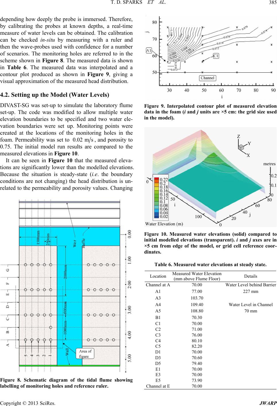

T. D. SPARKS ET AL. 385
depending how deeply the probe is immersed. Therefore,
by calibrating the probes at known depths, a real-time
measure of water levels can be obtained. The calibration
can be checked in-situ by measuring with a ruler and
then the wave-probes used with confidence for a number
of scenarios. The monitoring holes are referred to in the
scheme shown in Figure 8. The measured data is shown
in Table 6. The measured data was interpolated and a
contour plot produced as shown in Figure 9, giving a
visual approximation of the measured head distribution.
4.2. Setting up the Model (Water Levels)
DIVAST-SG was set-up to simulate the laboratory flume
set-up. The code was modified to allow multiple water
elevation boundaries to be specified and two water ele-
vation boundaries were set up. Monitoring points were
created at the locations of the monitoring holes in the
foam. Permeability was set to 0.02ms , and porosity to
0.75. The initial model run results are compared to the
measured elevations in Figure 10.
It can be seen in Figure 10 that the measured eleva-
tions are significantly lower than the modelled elevations.
Because the situation is steady-state (i.e. the boundary
conditions are not changing) the head distribution is un-
related to the permeability and porosity values. Changing
Figure 8. Schematic diagram of the tidal flume showing
labelling of monitoring holes and reference ruler.
Figure 9. Interpolated contour plot of measured elevation
data in the foam (i and j units are ×5 cm: the grid size used
in the model).
Figure 10. Measured water elevations (solid) compared to
initial modelled elevations (transparent). i and j axes are in
×5 cm from edge of the model, or grid cell reference coor-
dinates.
Table 6. Measured water elevations at steady state.
Location Measured Water Elevation
(mm above Flume Floor) Details
Channel at A70.00 Water Level behind Barrier
A1 77.00 227 mm
A3 103.70
A4 109.40 Water Level in Channel
A5 108.80 70 mm
B1 70.30
C1 70.00
C2 71.00
C3 76.00
C4 80.10
C5 82.20
D1 70.00
D3 70.60
D5 79.40
E1 70.00
E3 70.00
E5 73.90
Channel at E70.00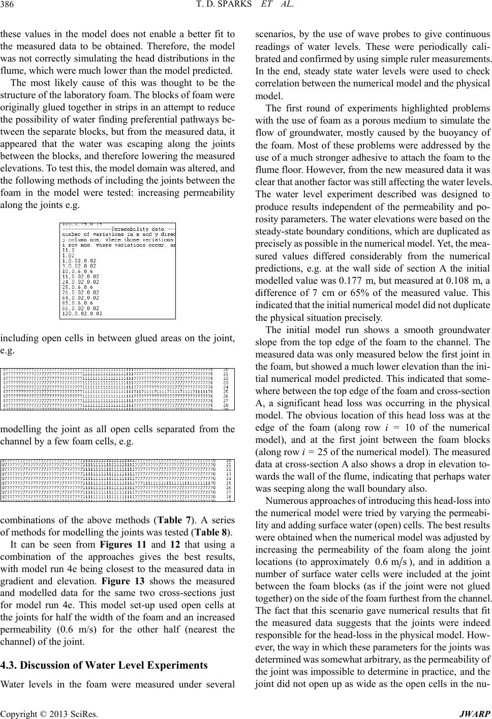

T. D. SPARKS ET AL. 386
these values in the model does not enable a better fit to
the measured data to be obtained. Therefore, the model
was not correctly simulating the head distributions in the
flume, which were much lower than the model predicted.
The most likely cause of this was thought to be the
structure of the laboratory foam. The blocks of foam were
originally glued together in strips in an attempt to reduce
the possibility of water finding preferential pathways be-
tween the separate blocks, but from the measured data, it
appeared that the water was escaping along the joints
between the blocks, and therefore lowering the measured
elevations. To test this, the model domain was altered, and
the following methods of including the joints between the
foam in the model were tested: increasing permeability
along the joints e.g.
including open cells in between glued areas on the joint,
e.g.
modelling the joint as all open cells separated from the
channel by a few foam cells, e.g.
combinations of the above methods (Table 7). A series
of methods for modelling the joints was tested (Table 8).
It can be seen from Figures 11 and 12 that using a
combination of the approaches gives the best results,
with model run 4e being closest to the measured data in
gradient and elevation. Figure 13 shows the measured
and modelled data for the same two cross-sections just
for model run 4e. This model set-up used open cells at
the joints for half the width of the foam and an increased
permeability (0.6 m/s) for the other half (nearest the
channel) of the joint.
4.3. Discussion of Water Level Experiments
Water levels in the foam were measured under several
scenarios, by the use of wave probes to give continuous
readings of water levels. These were periodically cali-
brated and confirmed by using simple ruler measurements.
In the end, steady state water levels were used to check
correlation between the numerical model and the physical
model.
The first round of experiments highlighted problems
with the use of foam as a porous medium to simulate the
flow of groundwater, mostly caused by the buoyancy of
the foam. Most of these problems were addressed by the
use of a much stronger adhesive to attach the foam to the
flume floor. However, from the new measured data it was
clear that another factor was still affecting the water levels.
The water level experiment described was designed to
produce results independent of the permeability and po-
rosity parameters. The water elevations were based on the
steady-state boundary conditions, which are duplicated as
precisely as possible in the numerical model. Yet, the mea-
sured values differed considerably from the numerical
predictions, e.g. at the wall side of section A the initial
modelled value was 0.177 m, but measured at 0.108 m, a
difference of 7 cm or 65% of the measured value. This
indicated that the initial numerical model did not duplicate
the physical situation precisely.
The initial model run shows a smooth groundwater
slope from the top edge of the foam to the channel. The
measured data was only measured below the first joint in
the foam, but showed a much lower elevation than the ini-
tial numerical model predicted. This indicated that some-
where between the top edge of the foam and cross-section
A, a significant head loss was occurring in the physical
model. The obvious location of this head loss was at the
edge of the foam (along row i = 10 of the numerical
model), and at the first joint between the foam blocks
(along row i = 25 of the numerical model). The measured
data at cross-section A also shows a drop in elevation to-
wards the wall of the flume, indicating that perhaps water
was seeping along the wall boundary also.
Numerous approaches of introducing this head-loss into
the numerical model were tried by varying the permeabi-
lity and adding surface water (open) cells. The best results
were obtained when the numerical model was adjusted by
increasing the permeability of the foam along the joint
locations (to approximately 0.6ms ), and in addition a
number of surface water cells were included at the joint
between the foam blocks (as if the joint were not glued
together) on the side of the foam furthest from the channel.
The fact that this scenario gave numerical results that fit
the measured data suggests that the joints were indeed
responsible for the head-loss in the physical model. How-
ever, the way in which these parameters for the joints was
determined was somewhat arbitrary, as the permeability of
the joint was impossible to determine in practice, and the
joint did not open up as wide as the open cells in the nu-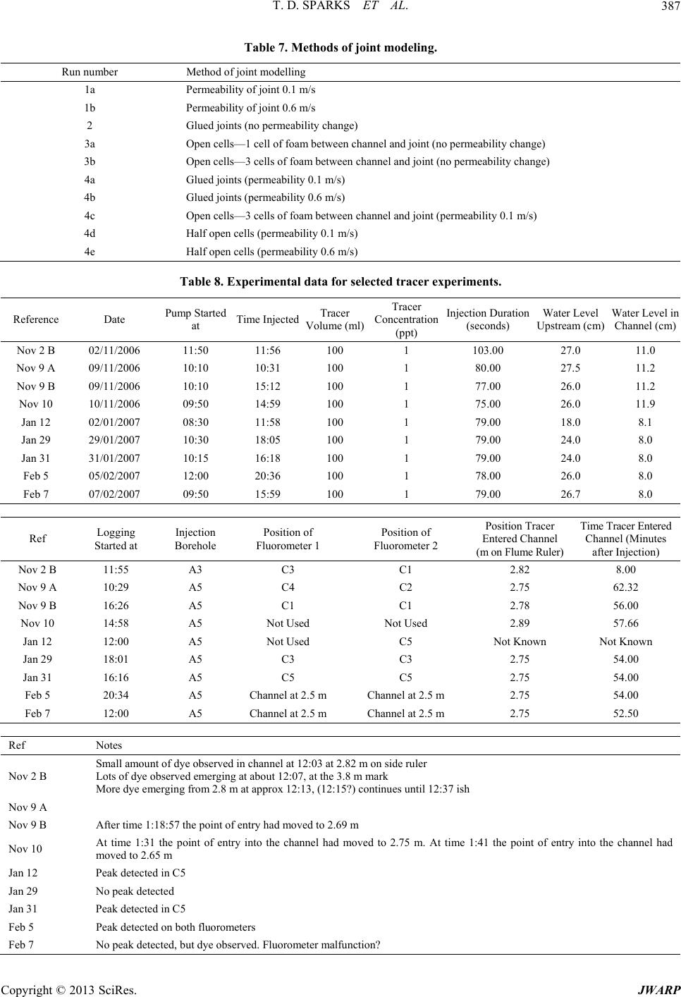

T. D. SPARKS ET AL. 387
Table 7. Methods of joint modeling.
Run number Method of joint modelling
1a Permeability of joint 0.1 m/s
1b Permeability of joint 0.6 m/s
2 Glued joints (no permeability change)
3a Open cells—1 cell of foam between channel and joint (no permeability change)
3b Open cells—3 cells of foam between channel and joint (no permeability change)
4a Glued joints (permeability 0.1 m/s)
4b Glued joints (permeability 0.6 m/s)
4c Open cells—3 cells of foam between channel and joint (permeability 0.1 m/s)
4d Half open cells (permeability 0.1 m/s)
4e Half open cells (permeability 0.6 m/s)
Table 8. Experimental data for selected tracer experiments.
Reference Date
Pump Started
at Time InjectedTracer Volume (ml)
Tracer
Concentration
(ppt)
Injection Duration
(seconds)
Water Level
Upstream (cm)
Water Level in
Channel (cm)
Nov 2 B 02/11/2006 11:50 11:56 100 1 103.00 27.0 11.0
Nov 9 A 09/11/2006 10:10 10:31 100 1 80.00 27.5 11.2
Nov 9 B 09/11/2006 10:10 15:12 100 1 77.00 26.0 11.2
Nov 10 10/11/2006 09:50 14:59 100 1 75.00 26.0 11.9
Jan 12 02/01/2007 08:30 11:58 100 1 79.00 18.0 8.1
Jan 29 29/01/2007 10:30 18:05 100 1 79.00 24.0 8.0
Jan 31 31/01/2007 10:15 16:18 100 1 79.00 24.0 8.0
Feb 5 05/02/2007 12:00 20:36 100 1 78.00 26.0 8.0
Feb 7 07/02/2007 09:50 15:59 100 1 79.00 26.7 8.0
Ref Logging
Started at
Injection
Borehole
Position of
Fluorometer 1
Position of
Fluorometer 2
Position Tracer
Entered Channel
(m on Flume Ruler)
Time Tracer Entered
Channel (Minutes
after Injection)
Nov 2 B 11:55 A3 C3 C1 2.82 8.00
Nov 9 A 10:29 A5 C4 C2 2.75 62.32
Nov 9 B 16:26 A5 C1 C1 2.78 56.00
Nov 10 14:58 A5 Not Used Not Used 2.89 57.66
Jan 12 12:00 A5 Not Used C5 Not Known Not Known
Jan 29 18:01 A5 C3 C3 2.75 54.00
Jan 31 16:16 A5 C5 C5 2.75 54.00
Feb 5 20:34 A5 Channel at 2.5 m Channel at 2.5 m 2.75 54.00
Feb 7 12:00 A5 Channel at 2.5 m Channel at 2.5 m 2.75 52.50
Ref Notes
Nov 2 B
Small amount of dye observed in channel at 12:03 at 2.82 m on side ruler
Lots of dye observed emerging at about 12:07, at the 3.8 m mark
More dye emerging from 2.8 m at approx 12:13, (12:15?) continues until 12:37 ish
Nov 9 A
Nov 9 B After time 1:18:57 the point of entry had moved to 2.69 m
Nov 10 At time 1:31 the point of entry into the channel had moved to 2.75 m. At time 1:41 the point of entry into the channel had
moved to 2.65 m
Jan 12 Peak detected in C5
Jan 29 No peak detected
Jan 31 Peak detected in C5
Feb 5 Peak detected on both fluorometers
Feb 7 No peak detected, but dye observed. Fluorometer malfunction?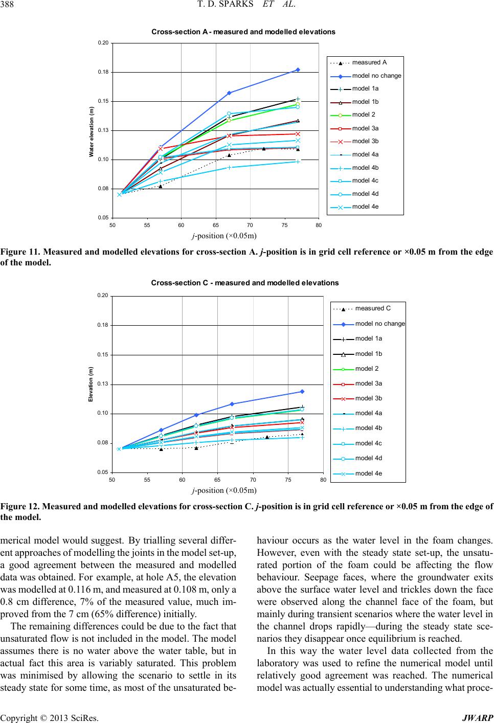

T. D. SPARKS ET AL. 388
Cross-section A - measured and m odelled elevations
0.05
0.08
0.10
0.13
0.15
0.18
0.20
50 5560 6570 7580
Water elevation (m)
meas ured A
mod el no change
model 1a
model 1b
model 2
model 3a
model 3b
model 4a
model 4b
model 4c
model 4d
model 4e
j-position (×0.05m)
Figure 11. Measured and modelled elevations for cross-section A. j-position is in grid cell reference or ×0.05 m from the edge
of the model.
Cross-section C - measured and modelled elevations
0.05
0.08
0.10
0.13
0.15
0.18
0.20
50 55 60 6570 75 80
Elevation (m)
meas ured C
model no change
model 1a
model 1b
model 2
model 3a
model 3b
model 4a
model 4b
model 4c
model 4d
model 4e
j-position (×0.05m)
Figure 12. Measured and modelled elevations for cross-section C. j-position is in grid cell refer ence or ×0 .05 m from the edge o f
the model.
merical model would suggest. By trialling several differ-
ent approaches of modelling the joints in the model set-up,
a good agreement between the measured and modelled
data was obtained. For example, at hole A5, the elevation
was modelled at 0.116 m, and measured at 0.108 m, only a
0.8 cm difference, 7% of the measured value, much im-
proved from the 7 cm (65% difference) initially.
The remaining differences could be due to the fact that
unsaturated flow is not included in the model. The model
assumes there is no water above the water table, but in
actual fact this area is variably saturated. This problem
was minimised by allowing the scenario to settle in its
steady state for some time, as most of the unsaturated be-
haviour occurs as the water level in the foam changes.
However, even with the steady state set-up, the unsatu-
rated portion of the foam could be affecting the flow
behaviour. Seepage faces, where the groundwater exits
above the surface water level and trickles down the face
were observed along the channel face of the foam, but
mainly during transient scenarios where the water level in
the channel drops rapidly—during the steady state sce-
narios they disappear once equilibrium is reached.
In this way the water level data collected from the
laboratory was used to refine the numerical model until
relatively good agreement was reached. The numerical
model was actually essential to understanding what proce-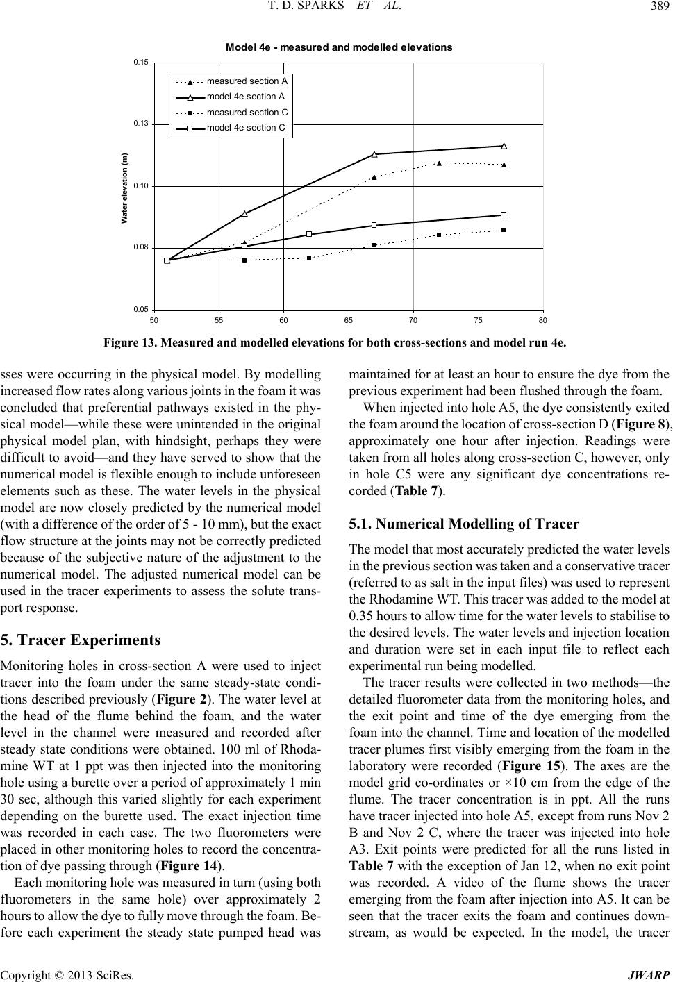

T. D. SPARKS ET AL. 389
Model 4e - measured and model led el evations
0.05
0.08
0.10
0.13
0.15
50 55 6065 70
Water elevation (m)
75 80
meas ured s ecti on A
model 4e sect ion A
meas ured s ecti on C
model 4e sect ion C
Figure 13. Measured and modelled elevations for both cross-sections and model run 4e.
sses were occurring in the physical model. By modelling
increased flow rates along various joints in the foam it was
concluded that preferential pathways existed in the phy-
sical model—while these were unintended in the original
physical model plan, with hindsight, perhaps they were
difficult to avoid—and they have served to show that the
numerical model is flexible enough to include unforeseen
elements such as these. The water levels in the physical
model are now closely predicted by the numerical model
(with a difference of the order of 5 - 10 mm), but the exact
flow structure at the joints may not be correctly predicted
because of the subjective nature of the adjustment to the
numerical model. The adjusted numerical model can be
used in the tracer experiments to assess the solute trans-
port response.
5. Tracer Experiments
Monitoring holes in cross-section A were used to inject
tracer into the foam under the same steady-state condi-
tions described previously (Figure 2). The water level at
the head of the flume behind the foam, and the water
level in the channel were measured and recorded after
steady state conditions were obtained. 100 ml of Rhoda-
mine WT at 1 ppt was then injected into the monitoring
hole using a burette over a period of approximately 1 min
30 sec, although this varied slightly for each experiment
depending on the burette used. The exact injection time
was recorded in each case. The two fluorometers were
placed in other monitoring holes to record the concentra-
tion of dye passing through (Figure 14).
Each monitoring hole was measured in turn (using both
fluorometers in the same hole) over approximately 2
hours to allow the dye to fully move through the foam. Be-
fore each experiment the steady state pumped head was
maintained for at least an hour to ensure the dye from the
previous experiment had been flushed through the foam.
When injected into hole A5, the dye consistently exited
the foam around the location of cross-section D (Figur e 8),
approximately one hour after injection. Readings were
taken from all holes along cross-section C, however, only
in hole C5 were any significant dye concentrations re-
corded (Table 7).
5.1. Numerical Modelling of Tracer
The model that most accurately predicted the water levels
in the previous section was taken and a conservative tracer
(referred to as salt in the input files) was used to represent
the Rhodamine WT. This tracer was added to the model at
0.35 hours to allow time for the water levels to stabilise to
the desired levels. The water levels and injection location
and duration were set in each input file to reflect each
experimental run being modelled.
The tracer results were collected in two methods—the
detailed fluorometer data from the monitoring holes, and
the exit point and time of the dye emerging from the
foam into the channel. Time and location of the modelled
tracer plumes first visibly emerging from the foam in the
laboratory were recorded (Figure 15). The axes are the
model grid co-ordinates or ×10 cm from the edge of the
flume. The tracer concentration is in ppt. All the runs
have tracer injected into hole A5, except from runs Nov 2
B and Nov 2 C, where the tracer was injected into hole
A3. Exit points were predicted for all the runs listed in
Table 7 with the exception of Jan 12, when no exit point
was recorded. A video of the flume shows the tracer
emerging from the foam after injection into A5. It can be
seen that the tracer exits the foam and continues down-
stream, as would be expected. In the model, the tracer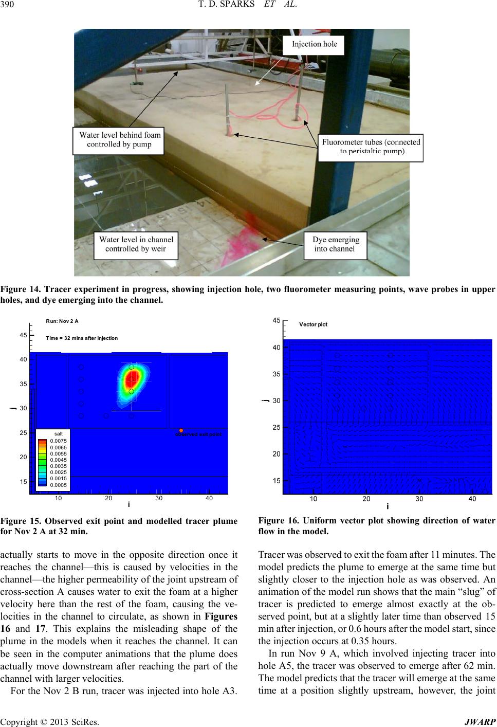

T. D. SPARKS ET AL. 390
Figure 14. Tracer experiment in progress, showing injection hole, two fluorometer measuring points, wave probes in upper
holes, and dye emerging into the channel.
i
j
10 20 30
15
20
25
30
35
40
45
salt
0.0075
0.0065
0.0055
0.0045
0.0035
0.0025
0.0015
0.0005
Time=32mins after injection
40
observed exitpoint
Run: Nov2 A
Figure 15. Observed exit point and modelled tracer plume
for Nov 2 A at 32 min.
actually starts to move in the opposite direction once it
reaches the channel—this is caused by velocities in the
channel—the higher permeability of the joint upstream of
cross-section A causes water to exit the foam at a higher
velocity here than the rest of the foam, causing the ve-
locities in the channel to circulate, as shown in Figures
16 and 17. This explains the misleading shape of the
plume in the models when it reaches the channel. It can
be seen in the computer animations that the plume does
actually move downstream after reaching the part of the
channel with larger velocities.
For the Nov 2 B run, tracer was injected into hole A3.
Figure 16. Uniform vector plot showing direction of water
flow in the model.
Tracer was observed to exit the foam after 11 minutes. The
model predicts the plume to emerge at the same time but
slightly closer to the injection hole as was observed. An
animation of the model run shows that the main “slug” of
tracer is predicted to emerge almost exactly at the ob-
served point, but at a slightly later time than observed 15
min after injection, or 0.6 hours after the model start, since
the injection occurs at 0.35 hours.
In run Nov 9 A, which involved injecting tracer into
hole A5, the tracer was observed to emerge after 62 min.
The model predicts that the tracer will emerge at the same
time at a position slightly upstream, however, the joint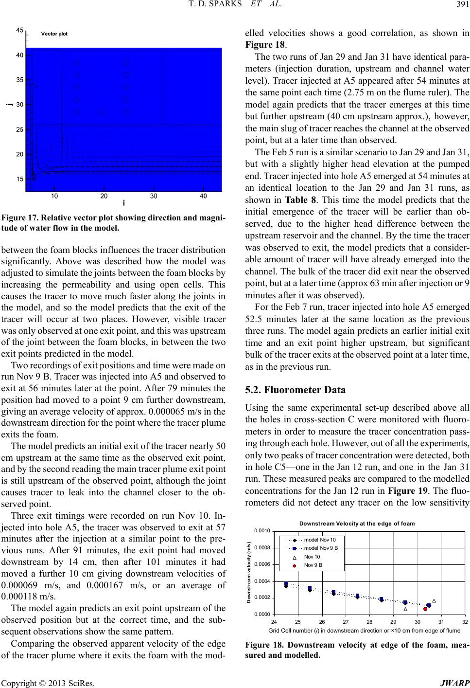

T. D. SPARKS ET AL. 391
Figure 17 . Relative vec tor plot s howing dir e ctio n and magni-
tude of water flow in the model.
between the foam blocks influences the tracer distribution
significantly. Above was described how the model was
adjusted to simulate the joints between the foam blocks by
increasing the permeability and using open cells. This
causes the tracer to move much faster along the joints in
the model, and so the model predicts that the exit of the
tracer will occur at two places. However, visible tracer
was only observed at one exit point, and this was upstream
of the joint between the foam blocks, in between the two
exit points predicted in the model.
Two recordings of exit positions and time were made on
run Nov 9 B. Tracer was injected into A5 and observed to
exit at 56 minutes later at the point. After 79 minutes the
position had moved to a point 9 cm further downstream,
giving an average velocity of approx. 0.000065 m/s in the
downstream direction for the point where the tracer plume
exits the foam.
The model predicts an initial exit of the tracer nearly 50
cm upstream at the same time as the observed exit point,
and by the second reading the main tracer plume exit point
is still upstream of the observed point, although the joint
causes tracer to leak into the channel closer to the ob-
served point.
Three exit timings were recorded on run Nov 10. In-
jected into hole A5, the tracer was observed to exit at 57
minutes after the injection at a similar point to the pre-
vious runs. After 91 minutes, the exit point had moved
downstream by 14 cm, then after 101 minutes it had
moved a further 10 cm giving downstream velocities of
0.000069 m/s, and 0.000167 m/s, or an average of
0.000118 m/s.
The model again predicts an exit point upstream of the
observed position but at the correct time, and the sub-
sequent observations show the same pattern.
Comparing the observed apparent velocity of the edge
of the tracer plume where it exits the foam with the mod-
elled velocities shows a good correlation, as shown in
Figure 18.
The two runs of Jan 29 and Jan 31 have identical para-
meters (injection duration, upstream and channel water
level). Tracer injected at A5 appeared after 54 minutes at
the same point each time (2.75 m on the flume ruler). The
model again predicts that the tracer emerges at this time
but further upstream (40 cm upstream approx.), however,
the main slug of tracer reaches the channel at the observed
point, but at a later time than observed.
The Feb 5 run is a similar scenario to Jan 29 and Jan 31,
but with a slightly higher head elevation at the pumped
end. Tracer injected into hole A5 emerged at 54 minutes at
an identical location to the Jan 29 and Jan 31 runs, as
shown in Table 8. This time the model predicts that the
initial emergence of the tracer will be earlier than ob-
served, due to the higher head difference between the
upstream reservoir and the channel. By the time the tracer
was observed to exit, the model predicts that a consider-
able amount of tracer will have already emerged into the
channel. The bulk of the tracer did exit near the observed
point, but at a later time (approx 63 min after injection or 9
minutes after it was observed).
For the Feb 7 run, tracer injected into hole A5 emerged
52.5 minutes later at the same location as the previous
three runs. The model again predicts an earlier initial exit
time and an exit point higher upstream, but significant
bulk of the tracer exits at the observed point at a later time,
as in the previous run.
5.2. Fluorometer Data
Using the same experimental set-up described above all
the holes in cross-section C were monitored with fluoro-
meters in order to measure the tracer concentration pass-
ing through each hole. However, out of all the experiments,
only two peaks of tracer concentration were detected, both
in hole C5—one in the Jan 12 run, and one in the Jan 31
run. These measured peaks are compared to the modelled
concentrations for the Jan 12 run in Figure 19. The fluo-
rometers did not detect any tracer on the low sensitivity
Downstream Velo cit y at the edg e of foam
0.0000
0.0002
0.0004
0.0006
0.0008
0.0010
24 2526 27 28 2930 31 32
Do w nst ream vel oci t y (m / s)
model Nov 10
model Nov 9 B
Nov 10
Nov 9 B
Grid Cell number (i) in downstream direction or ×10 cm from edge of flum e
Figure 18. Downstream velocity at edge of the foam, mea-
sured and modelled.

T. D. SPARKS ET AL.
Copyright © 20JWARP
392
setting, so in both cases the medium sensitivity setting
was used, meaning that concentrations over 1000 ppb
(0.001 ppt) were not measured. This meant that the peak
concentration was not recorded, but the timing of the
peak was still valid. The fluorometers were placed in the
channel for the Feb 5 run and both fluorometers detected
peaks in this run. The measured concentrations are plot-
ted against the modelled concentrations for the same
point in the channel in Figure 20.
pores on the edge of the hole were made more resistant to
flow, or perhaps the glue used to affix the plug into the
base of the hole blocked up some of the foam pores, mak-
ing a preferential flowpath around the monitoring hole.
However, this is thought unlikely as tracer was observed
in at least one of the monitoring holes;
b) The tracer could be travelling through the foam plug
at the base of the monitoring hole and so be undetected by
the fluorometer tube that takes a sample from the free
water in the hole. This is unlikely because the glue used to
secure the plug would, if anything, restrict flow through
this plug;
5.3. Discussion of Tracer Experiments
It was hoped to measure peaks of tracer concentration in
several different holes, but despite repeated experiments
and endless calibration and repair, only one hole yielded a
measurable peak. However, the tracer still exited the foam
at the expected place or relatively close to the expected
place. There could be a few reasons for this anomaly:
c) the tracer could be bypassing the monitoring hole by
short-circuiting underneath the foam or along the side of
the blocks, although this is again unlikely due to the glue
at the base of the foam securing it to the floor of the flume;
d) the tracer may not be evenly distributed over the
depth of the water column. The fluorometer sampling tube
necessarily only samples from one part of the water co-
lumn and could miss the tracer if it moves in a “layer”.
a) The tracer may not enter the monitoring hole at all
but move round the holes if there is any resistance to flow
into the hole itself. In cutting the hole perhaps the foam
Tracer Concentrat i on i n hole C5 for Jan 12
0
0.001
0.002
0.003
0.004
0.005
0.006
0.007
00.2 0.4 0.6 0.811.2 1.4 1.6
Time after injection (hours)
Tracer concentration (ppt)
mea s ured j an 12 - C5
es timat ed p eak
mod elled Jan 12 - C5
Figure 19. Tracer concentration in hole C5 for Jan 12.
13 SciRes.
Me asur ed a nd M odel led Tr a cer Concent r at ions i n t he Channel f or Feb 5
0.00025
0.00030
0.00035
2.50 3.00
n (pp t)
0.00000
0.00005
0.00010
0.00015
0.00020
0.00 0.50 1.001.50 2.00
Time a fter Injection (hours)
Tracer Con cen trati o
measured feb 5 f l1 c hann el
measured feb 5 f l2 c hann el
model l ed f eb 5 ch ann el
Figure 20. Tracer concentration in the channel (2.5 m on ruler) for Feb 5.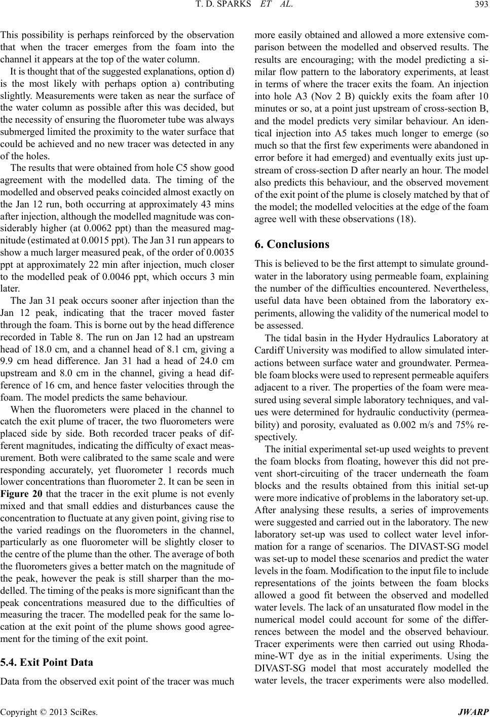

T. D. SPARKS ET AL. 393
This possibility is perhaps reinforced by the observation
that when the tracer emerges from the foam into the
channel it appears at the top of the water column.
It is thought that of the suggested explanations, option d)
is the most likely with perhaps option a) contributing
slightly. Measurements were taken as near the surface of
the water column as possible after this was decided, but
the necessity of ensuring the fluorometer tube was always
submerged limited the proximity to the water surface that
could be achieved and no new tracer was detected in any
of the holes.
The results that were obtained from hole C5 show good
agreement with the modelled data. The timing of the
modelled and observed peaks coincided almost exactly on
the Jan 12 run, both occurring at approximately 43 mins
after injection, although the modelled magnitude was con-
siderably higher (at 0.0062 ppt) than the measured mag-
nitude (estimated at 0.0015 ppt). The Jan 31 run appears to
show a much larger measured peak, of the order of 0.0035
ppt at approximately 22 min after injection, much closer
to the modelled peak of 0.0046 ppt, which occurs 3 min
later.
The Jan 31 peak occurs sooner after injection than the
Jan 12 peak, indicating that the tracer moved faster
through the foam. This is borne out by the head difference
recorded in Table 8. The run on Jan 12 had an upstream
head of 18.0 cm, and a channel head of 8.1 cm, giving a
9.9 cm head difference. Jan 31 had a head of 24.0 cm
upstream and 8.0 cm in the channel, giving a head dif-
ference of 16 cm, and hence faster velocities through the
foam. The model predicts the same behaviour.
When the fluorometers were placed in the channel to
catch the exit plume of tracer, the two fluorometers were
placed side by side. Both recorded tracer peaks of dif-
ferent magnitudes, indicating the difficulty of exact meas-
urement. Both were calibrated to the same scale and were
responding accurately, yet fluorometer 1 records much
lower concentrations than fluorometer 2. It can be seen in
Figure 20 that the tracer in the exit plume is not evenly
mixed and that small eddies and disturbances cause the
concentration to fluctuate at any given point, giving rise to
the varied readings on the fluorometers in the channel,
particularly as one fluorometer will be slightly closer to
the centre of the plume than the other. The average of both
the fluorometers gives a better match on the magnitude of
the peak, however the peak is still sharper than the mo-
delled. The timing of the peaks is more significant than the
peak concentrations measured due to the difficulties of
measuring the tracer. The modelled peak for the same lo-
cation at the exit point of the plume shows good agree-
ment for the timing of the exit point.
5.4. Exit Point Data
Data from the observed exit point of the tracer was much
more easily obtained and allowed a more extensive com-
parison between the modelled and observed results. The
results are encouraging; with the model predicting a si-
milar flow pattern to the laboratory experiments, at least
in terms of where the tracer exits the foam. An injection
into hole A3 (Nov 2 B) quickly exits the foam after 10
minutes or so, at a point just upstream of cross-section B,
and the model predicts very similar behaviour. An iden-
tical injection into A5 takes much longer to emerge (so
much so that the first few experiments were abandoned in
error before it had emerged) and eventually exits just up-
stream of cross-section D after nearly an hour. The model
also predicts this behaviour, and the observed movement
of the exit point of the plume is closely matched by that of
the model; the modelled velocities at the edge of the foam
agree well with these observations (18).
6. Conclusions
This is believed to be the first attempt to simulate ground-
water in the laboratory using permeable foam, explaining
the number of the difficulties encountered. Nevertheless,
useful data have been obtained from the laboratory ex-
periments, allowing the validity of the numerical model to
be assessed.
The tidal basin in the Hyder Hydraulics Laboratory at
Cardiff University was modified to allow simulated inter-
actions between surface water and groundwater. Permea-
ble foam blocks were used to represent permeable aquifers
adjacent to a river. The properties of the foam were mea-
sured using several simple laboratory techniques, and val-
ues were determined for hydraulic conductivity (permea-
bility) and porosity, evaluated as 0.002 m/s and 75% re-
spectively.
The initial experimental set-up used weights to prevent
the foam blocks from floating, however this did not pre-
vent short-circuiting of the tracer underneath the foam
blocks and the results obtained from this initial set-up
were more indicative of problems in the laboratory set-up.
After analysing these results, a series of improvements
were suggested and carried out in the laboratory. The new
laboratory set-up was used to collect water level infor-
mation for a range of scenarios. The DIVAST-SG model
was set-up to model these scenarios and predict the water
levels in the foam. Modification to the input file to include
representations of the joints between the foam blocks
allowed a good fit between the observed and modelled
water levels. The lack of an unsaturated flow model in the
numerical model could account for some of the differ-
rences between the model and the observed behaviour.
Tracer experiments were then carried out using Rhoda-
mine-WT dye as in the initial experiments. Using the
DIVAST-SG model that most accurately modelled the
water levels, the tracer experiments were also modelled.

T. D. SPARKS ET AL. 394
Tracer proved difficult to measure in the foam boreholes
for a variety of possible reasons, however the results that
were obtained agreed well with the model. Encouraging
correlation was observed between the observed exit point
of the tracer from the foam, and the modelled exit point
and time.
7. Acknowledgements
The work carried out in this paper was supported by
NERC studentship NER/S/A/2003/11216.
REFERENCES
[1] H. H. J. Cooper and M. I. Rorabaugh, “Ground-Water
Movements and Bank Storage Due to Flood Stages in
Surface Streams,” US Geological Survey, 1963.
[2] G. F. Pinder and S. P. Sauer, “Numerical Simulation of
Flood Wave Modification Due to Bank Storage Effects,”
Water Resources Research, Vol. 7, No. 1, 1971, pp. 63-
70. doi:10.1029/WR007i001p00063
[3] R. E. Smith and D. A. Woolhiser, “Overland Flow on an
Infiltrating Surface,” Water Resources Research, Vol. 7,
No. 4, 1971, pp. 899-913.
doi:10.1029/WR007i004p00899
[4] R. Freeze and J. A. Cherry, “Groundwater,” Prentice-Hall,
Inc., Upper Saddle River, 1979.
[5] M. G. McDonald and A. W. Harbaugh, “A Modular
Three-Dimensional Finite Difference Ground-Water Flow
Model,” US Geological Survey, 1988.
[6] H. E. Jobson and A. W. Harbaugh, “Modifications to the
Diffusion Analogy Surface-Water Flow Model (DAFLOW)
for Coupling to the Modular Finite-Difference Ground-
Water Flow Model (MODFLOW),” US Geological Sur-
vey, Reston, 1999.
[7] M. L. Merrit and L. F. Konikow, “Documentation of a
Computer Program to Simulate Lake-Aquifer Interaction
Using the MODFLOW Ground-Water Flow Model and
the MOC3D Solute-Transport Model,” US Geological
Survey, Tallahassee, 2000.
[8] J. I. Restrepo, A. M. Montoya and J. Obeysekera, “A
Wetland Simulation Module for the MODFLOW Ground
Water Model,” Ground Water, Vol. 36, No. 5, 1998, pp.
764-770. doi:10.1111/j.1745-6584.1998.tb02193.x
[9] S. Panday and P. S. Huyakorn, “A Fully Coupled Physi-
cally-Based Spatially-Distributed Model for Evaluating
Surface/Subsurface Flow,” Advances in Water Resources,
Vol. 27, 2004, pp. 361-382.
doi:10.1016/j.advwatres.2004.02.016
[10] R. A. Falconer, “An Introduction to Nearly Horizontal
Flows,” In: M. B. Abbott and W. A. Price, Eds., Coastal,
Estuarial and Harbour Engineers’ Reference Book, E. &
F. N. Spoon Ltd., London, 1993, pp. 27-36.
[11] R. A. Falconer, B. Lin, Y. Wu and E. Harris, “DIVAST
Reference Manual,” Hydro-Environmental Research Cen-
tre, Cardiff University, Cardiff, 2001.
[12] R. A. Falconer, B. Lin, Y. Wu and E. Harris, “DIVAST
User Manual,” Hydro-Environmental Research Centre,
Cardiff University, Cardiff, 2001.
[13] T. Sparks, D. Kountcheva, B. Bockelmann and R. Fal-
coner, “Physical and Numerical Modelling of Groundwa-
ter and Surface-Water Interactions with a Conservative
Tracer,” ISSMGE Proceedings of 5th International Con-
gress on Environmental Geotechnics, Cardiff, June 2006.
[14] J. Baer, “Dynamics of Fluids in Porous Media,” Ameri-
can Elsevier Publishing Company Inc., New York, 1972.
[15] H. Darcy, “Les Fontaines Publiques de la Ville de Dijon,”
Dalmont, Paris, 1856.
[16] K. Spanoudaki, A. Nanou, A. I. Stamou, G. Christodou-
lou, T. Sparks, B. Bockelmann and R. A. Falconer, “Inte-
grated Surface Water-Groundwater Modelling,” Global
Network of Environmental Science and Technology (NEST)
Journal, Vol. 7, No. 3, 2005.
[17] EC, “Directive 2000/60/EC of the European Parliament
and of the Council of 23 October 2000 Establishing a
Framework for Community Action in the Field of Water
Policy,” European Parliament and Council 2000/60/EC,
2000.
[18] BS1377, “Determination of Permeability by the Constant-
Head Method,” British Standards, Part 5, 1990.
[19] J. Dupuit, “Études Théoriques et Pratiques sur le Mouve-
ment des eaux,” Dunos, Paris, 1863.
[20] H. Rouse, “Engineering Hydraulics,” John Wiley & Sons,
Inc., Hoboken, 1950.
[21] Turner_Designs, “Application Support Bulletin 103: Fluo-
rescein and a Fluorometer,” 2006.
http://www.turnerdesigns.com/t2/doc/appnotes/998_5103.
html
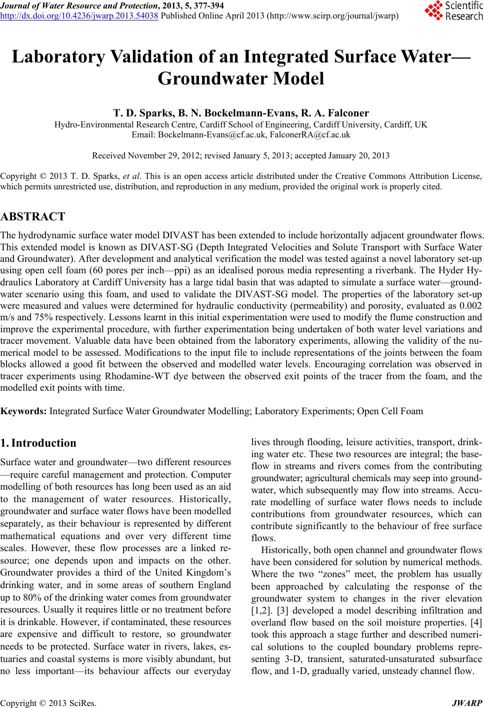