iBusiness, 2013, 5, 23-26
doi:10.4236/ib.2013.51b005 Published Online March 2013 (http://www.scirp.org/journal/ib)
23
Optimization of Tracking Error for Robust Portfolio of
Risk Assets with Trans ac t ion Cost
Dong Zheng, Xi-kun Liang
Hangzhou Institute of Service Engineering, Hangzhou Normal University, Hangzhou, China.
Received 2013
ABSTRACT
Based on the optimization of robust portfolio with tracking error, a robust mean-variance portfolio selection model of
tracking error with transaction cost is presented for the case that only risky assets exist and expected returns of assets
are uncertain and belong to a convex polyhedron. This paper aims to solve the problem of the portfolio with the selec-
tion o f the rat io on the c onditi on of ma ximumi mum fluc tuation o f the tra cking e rror, mak ing the e xpectat ion of t he re-
turn to be the maximumimum. It also makes the portfolio ’s practica l c ho ic e by the function of the linear transaction co st
as the same time of construction and application of the model. Empirical analysis with five real stocks is performed by
the metho d o f LMI (Linear Matrix Inequality) to show the efficiency of the model.
Keywords: Transaction Co st; T r a c king Error; Robust; Risk y Assets; Portfolio Optimizatio n
1. Introduction
The Mean-Variance model developed by Markowitz [1]
has been playing an important role in the field of asset
allocation. Based on this theory, some robust portfolio
optimization methods later has made up it effectively
[2-11]. Ben has researched the topic of the robust opti-
mization method and applications [2]. Pinara has studied
the issue about the robust profit opportunities in risky
financial portfolios [7]. On the condition of the separa-
tion of ownership of the funds and the rights of invest-
ment and management in the recent financial trading
market, the model of tracking error robust portfolio op-
timization has been applied in the practice of financial
investment: Assuming the situation that both the rate of
expected returns and the covariance matrix is uncertain
which belong to the known convex combinations, Costa
has studied the issue about tracking error robust portfolio
with the method of the linear-matrix inequalities [12].
Moreo ver, robust po rtfolio sel ection with transac tion co st
has been given high priority: Bertsimas[13] has re-
searched about robust multiperiod portfolio management
in the presence of transaction cost. Xue [14] has studied
about mean-variance portfolio optimal problem under
concave transaction cost and Erdogany [15] has studied
the issue about ro bust active portfolio management.
In this paper, we have researched the topic of tracking
error robust portfolio of risky assets with transaction cost
on the condition of the uncertainty of both the expected
return rate and the covariance matrix belonging to the
known con ve x set s. In t he e nd of th is pa per , an e mpirical
analysis is given through the method of LMI (Linear
Matrix Inequa lity) to show the efficiency of the model.
2. Introdution to Parameters
It is assumed that there are only n risky assets in the
market and which c an be writ ten as
( )
12
,,
n
A aaa=
.
a) The weight vector of the risky portfolio is
( )
12
,,, '
n
z zzz=
where
( )
12
,,, '
n
zz z is the transpose of
( )
12
,,,
n
zz z.
i
z
is the weight of portfolio in the
i th−
assets,
01, 1,2,,
i
zi n
≤≤= , and it satisfied with
'1zI⋅=
in
which
I
is the n-di me nsiona l uni t colu mn ve ct or .
b) The rate of the return vector of the risky assets can
be expressed as
( )
12
,, ,'
n
r rrr=
, where the transpose
of
( )
12
,,,
n
rr r
is
( )
12
,, ,'
n
rr r.
c) The rate of the expected return vector of the risky
assets can be written as:
( )
12
(),, ,'
n
Er µ µµµ = =
.
while the covariance matrix is noted as
nn
GR
×
∈
.
d) The vector of the transaction cost can be noted as:
11 21
()( ( ),( ),,())'
nn
PzPzPzP z=
,
where
()
ii
Pz is the individual transaction cost on the
i th−
risky ass et.
e) The net weight vector of po r tfolio is
( )
12
(), , ,'
n
zzPzz zz=−=
 

,

Optimization of Tracking Error for Robust Portfolio of Risk Assets with Transaction Cost
24
where
()
ii ii
zz Pz= −

is denoted for the weights of the
i th−
risky ass ets with tr ansact i on c ost.
f) The sum of the returns can be expressed as:
1
() '.
n
ii
i
R zzuz
µ
µ
=
== ∑
g) T he net of the returns of the risky assets can be de-
noted as
11
( )(())
nn
i
uiii ii
ii
NRzu zuzPz
= =
= =−
∑∑

(1)
h) The variance of the net returns of the portfolio can
be written as:

2
() 'z zGz σ =

(2)
i) The function of linear transaction cost of the risky
assets can be expressed as:
(),1, 2,,
i iiii
P zazbin=+=
As the fixed cost can be omitted, the above formula
can be simplified for
( ),01
i iiii
P zaza= <<
(3)
3. Tracking Error Robust Portfolio
Optimization under Certain Condition
Tracking error can be actually called for the difference
between the return of the investor’s portfolio and bench-
mark return portfolio. It can be assumed that the vector
of the predetermined benchmark return is
( )
12
, ,,'
n
B BBB
z zzz=
here. Usually, the tracking error
can be expressed either as the relative return
( )
() '
B
zzz u β = −
or as the variance
( )( )
2()'
BB
zzz Gzz σ =−−
.
Actually, it can be written into two situations which
are equal with each other in the optimization of the
tracking error: the first situation is to minimum the va-
riance in the condition of guaranting the fixed objective
of the relative return, the second situation is to maximum
the return under guaranting fixed the relative variance.
The model of the second situation can be expressed as
[12]
22
0
max( )
..( )
z
z
st z
z
β
σσ


≤

∈Ψ


(4)
4. Tracking Error Robust Portfolio
Optimization in Uncertain Market
The uncertain condition here is that both the expected
return and the covariance can be variable with the change
of the environment of the financial market. Costa as-
sumed that the parameter
µ
and
G
belong to two
different convex combinations respectively to describe
the uncertain[12], it can be written as
{ }
12
,,,
t
uCon uuu∈
,
{ }
12
,,,
t
GCon GGG∈
where 12
(,,, )',,1,2,,
kk kknk
uuuu Gkt= =
are stood
for the expected return and the covariance rerespectively
under the uncertain condition which are obtained by the
different methods.
The reference [12] demo nstrates the form of the linear
matrix inequalities to denote for the optimization in the
uncertain condition of the tracking error robust portfolio
with n risky assets and 1 risk-free asset based on the
condition above, so we can get robust portfolio optimiza-
tion with n risky assets through the model above as fol-
lows:
1
min
( )'
.. 0
()
() ',1, 2,,
1
01,1, 2,,
z
k Bk
kB k
Bk
n
i
i
i
zz G
st Gzz G
zz ukt
z
zi n
β
α
β
=
−

−

≥

−


− ≥=


=

≤≤ =


∑


(5)
where
max()' ,1,2,...
Bk
k
zzukt β =−=
has introduced
the bounded variable of the deviationist fluctuations, the
function of the model is to get the vector of weight of the
portfolio z to satisfy the condition of the maximum ex-
pected return
β
. The significance of mathematical
finance is to find a portfolio with maximum worst case
expected performance about a benchmark, with guaran-
teed fixed maximum tracking error volatility. Actually,
the maximum re turn ca n be writt en as:

{ }
min max()';()
Bk
zkzz uz
βα
=−− −∈Λ
where
{ }
();()'( )0,1,2,,
kBk B
zzzGzzkt αα Λ=∈Ψ− −−≥=
and
()'()0
kBkB
zz Gzz
α −−− ≥ can be obtained by the
method of Schur complement, 12 ( ,,...,)'
kt
α αα α = is
the vector of maximum volatility of the tracking error in
uncer t ain eco nomy of the future[12].
5. Tracking Error Robust Portfolio
Optimization of Risky Assets with
Transaction Cost
Based on model (5) above, we consider the linear trans-
action cost to bulid a new model of tracking errof robust
portfolio optimization of risky assets with transaction
cost. T his model is express as follo wing formula.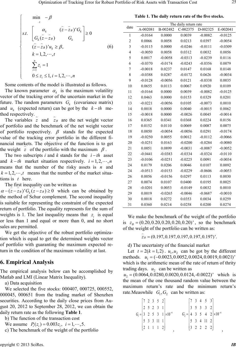

Optimization of Tracking Error for Robust Portfolio of Risk Assets with Transaction Cost
opyright © 2013 SciRes. IB
25
1
min
( )'
.. 0
()
( )',
1,2,,
1
01,1, 2,,
z
B
kk
B
kk
Bk
n
i
i
i
zz G
st Gzz G
zz u
kt
z
zi n
β
α
β
=
−



−
≥

−



−≥

=

=


≤≤ =

∑





(6)
So me c ontents of the model is illustrated as follo ws.
The known parameter
k
α
is the maximum volatility
vector of the tracking error of the uncertain market in the
future. The random parameters
k
G
(covariance matrix)
and k u (expected return) can be got by the k th− me-
thod respectively.
The variables
z

and B
z

are the net weight vector
of portfolio and the benchmark of the net weight vector
of portfolio respectively.
β
stands for the expected
value of the tracking error portfolio in the different fi-
nancial markets. The objective of the function is to get
the wei ght
z

of the portfolio with the maximum
β
.
The two subscripts i and k stands for the
i th−
asset
and
k th−
market situation respectively.
1, 2,,in=
means that the number of the risky assets is
n
and
1, 2,,kt=
means that the number of the market situa-
tions is
t
here.
The first inequality can be written as
()'()0
BB
k
zz Gzz α −−−≥
 
which can be obtained by
the method of Schur complement. The second inequality
is suitable for representing the constraint of the expected
return of portfolio. The equality represents for the sum of
weights is 1. The last inequality means that
i
z
is equal
or less than 1 and equal or more than 0, and no short
sales are permitted.
We get the objective of the robust portfolio optimiza-
tion which is equal to get the determined weights vector
of portfolio with guaranting the maximum expected re-
turn in the condition of the maximum vola tility at last.
6. Empirical Analysis
The empirical analysis below can be accomplished by
Matlab and LMI (Linear Matrix Inequality).
a) Data acq uisition
We selected the five stocks: 000407, 000725, 000552,
000045, 000651 from the trading market of Shenzhen
securities. According to the daily close prices from Au-
gust 20, 2012 to September 28, 2012, we can obtain the
daily return rate as the following Table 1.
b) The function of the t ra ns action cost
We assume
()0.003 ,1,,5.
ii i
Pzz i== 
c) The benchmark of the weight of the portfolio
Table 1. The daily retu rn rate of the five stocks.
date The daily return rate
A-002081 B-002482 C-002375 D-002325 E-002041
1 -0.0164 0.0000 0.0039 -0.0082 -0.0125
2 0.0066 0.0058 0.0213 0.0397 -0.0054
3 -0.0115 0.0000 -0.0246 -0.0111 -0.0309
4 -0.0050 0.0058 0.0312 0.0032 0.0056
5 0.0017 -0.0058 -0.0313 -0.0239 0.0116
6 -0.0370 -0.0174 -0.0243 -0.0356 0.0079
7 -0.0018 0.0237 0.0147 0.0168 0.0148
8 -0.0388 0.0287 -0.0172 0.0626 -0.0034
9 -0.0128 -0.0056 0.0121 -0.0338 0.0035
10 0.0655 0.0113 0.0067 0.0920 0.0109
11 -0. 0164 0.0000 0.0039 -0.0082 -0.012 5
12 0.0463 0.0000 0.0153 0.0329 0.0201
13 -0. 0221 -0.0056 0.0105 -0.0073 0.0010
14 0.0018 0.0000 0.0040 -0.0015 0.0062
15 -0. 0018 0.0000 -0.0026 0.0045 -0.0014
16 0.0365 0.0341 0.0368 0.0224 0.0156
17 0.0152 0.0110 0.0069 0.0087 0.0075
18 0.0050 -0.0054 -0.0056 0.0291 -0.0174
19 -0. 0250 0.0055 0.0012 -0.0112 -0.006 6
20 -0. 0251 0.0163 -0.0200 -0.028 4 -0.0080
21 0.0051 0.0899 -0.0031 -0.0087 -0.0052
22 -0. 0441 -0.0383 -0.0334 -0.0324 -0.0110
23 -0. 0106 -0.0251 -0.0225 0.0091 -0.0034
24 0.0179 0.0206 0.0046 0.0107 0.0092
24 -0.0513 -0. 0153 -0.0229 -0.0606 -0.0053
26 0.0056 -0.0156 0.0297 0.0113 0.0030
27 0.0074 0.0107 0.0400 0.0195 0.0025
28 -0.0201 0.0053 -0.0149 0.0032 0.0010
29 0.0019 -0.0265 -0.0046 -0.0687 -0.0010
30 0.0018 0.0272 0.0353 0.0034 0.0259
31 0.0360 0.0214 0.0258 0.0200 0.0274
We make the benchmark of the weight of the portfolio
is (0.20,0.20,0.20,0.20,0.20)'
B
z=, so the benchmark
of the weight of the portfolio c a n b e written as:
(0.197,0.197,0.197,0.197,0.197)'.
B
z=

d) The uncert ainty of the financial market
Let 2( 1,2)tk= =.
12
,uu
can be got by the different
methods.
1
( 0.0023,0.0052,0.0024,0.0019,0.0021)'u=−
which is the arithmetic mean of the rate of return of thrit y
trading days. 2 u can be written as
2
(0.0064,0.0280,0.0020,0.0124,-0.0022)'u=
which is
the mean of the one tho usand random value between t he
maximum return’s rate and the minimum return’s
rate.Measwhile
12
,
GG
can be written as:
4
1
72352
25231
10 325 31
53311 1
211 1 2
G
−




= ×




,
4
2
73453
35332
10
435 4 2
534112
32222
G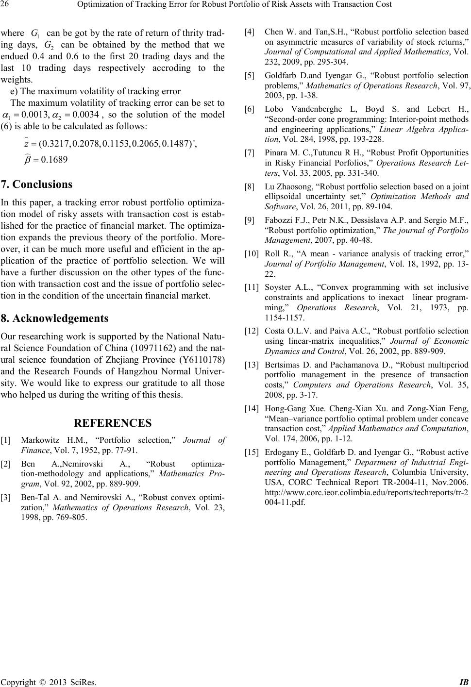
−




= ×




,

Optimization of Tracking Error for Robust Portfolio of Risk Assets with Transaction Cost
26
where
1
G
can b e got by the r ate of ret urn o f thrit y trad-
ing days,
2
G
can be obtained by the method that we
endued 0.4 and 0.6 to the first 20 trading days and the
last 10 trading days respectively accroding to the
weig h ts.
e) The max i mu m volat ility of tra c king er ror
The maximu m volatility of tra cking error can be set to
12
0.0013, 0.0034 αα = =
, so the solution of the model
(6) is able to be calculated as follows:

(0.3217,0.2078,0.1153,0.2065,0.1487)',
0.1689
z
β
=
=

7. Conclusions
In this paper, a tracking error robust portfolio optimiza-
tion model of risky assets with transaction cost is estab-
lished for the pr actice of financial market. T he optimiza-
tion expands the previous theory of the portfolio. More-
over, it can be much more useful and efficient in the ap-
plication of the practice of portfolio selection. We will
have a further discussion on the other types of the func-
tion with transactio n cost and the issue o f portfolio selec-
tion in the condition of the uncertain financial market.
8. Acknowledgemen ts
Our researching work is supported by the National Natu-
ral S cience Fo undatio n of China ( 109711 62) and the nat-
ural science foundation of Zhejiang Province (Y6110178)
and the Research Founds of Hangzhou Normal Univer-
sity. We would like to express our gratitude to all those
who he lped us duri ng t he writi ng of this thesis.
REFERENCES
[1] Markowitz H.M., “Portfolio selection,” Journal of
Finance, Vol. 7, 1952, pp. 77-91.
[2] Ben A.,Nemirovski A., “Robust optimiza-
tion-methodology and applications,” Mathematics Pro-
gram, Vol. 92, 2002, pp. 889-909.
[3] Ben -Tal A. and Nemirovski A., “Robust convex optimi-
zation,” Mathematics of Operations Research, Vol. 23,
1998, pp. 769-805.
[4] Chen W. and Tan,S.H., “Robust portfolio selection based
on asymmetric measures of variability of stock returns,”
Journal of Computational and Applied Mathematics, Vol.
232, 2009, pp. 295-304.
[5] Goldfarb D.and Iyengar G., “Robust portfolio selection
problems,” Mathematics of Operations Research, Vol. 97,
2003, pp. 1-38.
[6] Lobo Vandenberghe L, Boyd S. and Lebert H.,
“Secon d-order cone programming: Interior-point methods
and engineering applications,” Linear Algebra Applica-
tion, Vol. 284, 1998, pp. 193-228.
[7] Pinara M. C.,Tutuncu R H., “Robust Profit Opportunities
in Risky Financial Porfolios,” Operations Research Let-
ters, Vol. 33, 2005, pp. 331-340.
[8] Lu Zhaosong, “Robust portfolio selection based on a joint
ellipsoidal uncertainty set,” Optimization Methods and
Software, Vol. 26, 2011, pp. 89-104.
[9] Fab ozzi F.J. , Petr N.K., D essislava A.P . and Sergio M.F.,
“Robust portfolio optimization,” The journal of Portfolio
Management, 2007, pp. 40-48.
[10] Roll R., “A mean - variance analysis of tracking error,”
Journal of Portfolio Management, Vol. 18, 1992, pp. 13-
22.
[11] Soyster A.L., “Convex programming with set inclusive
constraints and applications to inexact linear program-
ming,” Operations Research, Vol. 21, 1973, pp.
1154-1157.
[12] Costa O.L.V . and Pai va A.C., “R obust portfolio selectio n
using linear-matrix inequalities,” Journal of Economic
Dynamics and Control, Vol. 26, 2002, pp. 889-909.
[13] Bertsimas D. and Pachamanova D., “Robust multiperiod
portfolio management in the presence of transaction
costs,” Computers and Operations Research, Vol. 35,
2008, pp. 3-17.
[14] Hong-Gang Xue. Cheng-Xian Xu. and Zong-Xian Feng,
“Mean–variance portfolio optimal problem under concave
transact ion co st,” Applied Mathematics and Computation,
Vol. 174, 2006, pp. 1-12.
[15] Erdogany E., Goldfarb D. and Iyengar G., “Robust active
portfolio Management,” Department of Industrial Engi-
neering and Operations Research, Columbia University,
USA, CORC Technical Report TR-2004-11, Nov.2006.
http://www.corc.ieor.colimbia.edu/reports/techreports/tr-2
004-11.pdf.