Journal of Software Engineering and Applications, 2013, 6, 1-3
doi:10.4236/jsea.2013.63b001 Published Online March 2013 (http://www.scirp.org/journal/jsea)
1
Research on Fault Prediction of Modern Aviation
Electronic Equipment Based on Improved Grey Model
Junjie Zhou1, Qigen Jing1, Xinhua Xie1, Naidong Zhou2
1Unit 95926, Aviation University of Air Force, Chang Chun, China; 2Equipment Department of Unit 95988, Aviation University of
Air Force, Chang Chun, China.
Received 2013
ABSTRACT
The basic principle and method of Grey Model prediction are presented. In view of the defects of general GM(1,1)
model, an improved method is proposed. That is using the particle swarm optimization algorithm to obtain the best
forecast dimension and using metabolism to make the model parameters adaptively change. Finally, the improved Grey
Model is used to predict the fault of high voltage power supply circuit of a certain type of modern air-borne radar. The
results which are computed and simulated by Matlab software show that the forecast precision of improved Grey Model
is higher than that of original Grey Model.
Keywords: Grey Model; Fault Prediction; Modern Aviation Electronic Equipment
1. Introduction
With all kinds of high technology such as the microelec-
tronic and artificial intelligence applied in modern avia-
tion electronic equipment, its integration and complexity
are greatly improved. Traditional maintenance mode,
such as the breakdown maintenance and preventive
maintenance, has not been adap ted to it. Condition based
maintenance which requires that the equipment itself
must have the ability to predict fault will replace tradi-
tional maintenance mode because of its good economic
affordability and small maintenance scale.
Compared with traditional maintenance mode, condi-
tion based maintenance which enabled system or com-
ponents of modern aviation electronic equipment to find
fault before it happened is more scientific and advisable.
So we can see that fault prediction is the critical tech-
nology to realize condition based maintenance.
Because of the complex system composition, fuzzy
structure and limited characteristic parameters, it’s hard
to predict the fault of modern aviation electronic equip-
ment. Grey Model which supplies a new way to resolve
the problems of sub-sample, poor information and un-
certainty is an effective measure to predict its fault.
2. Basic Principle of Grey Model Prediction
The grey system theory, which is proposed by Professor
Julong Deng in 1982, is used in studying of uncertain
system with features of sub-sa mple and poor information.
Its most prominent feature is to model with small data.
The GM(1,1) model is one of the important contents in
grey system theory and it has been widely used in many
fields including fault prediction [1].
2.1. Accumulated Generating Operation (AGO)
Suppose the original sequence is:
(0)(0) (0)(0)
{(1),(2),,()},
X
xx xn…
The first order AGO sequence is:
(1)(1) (1)(1)
{(1),(2),,()}
X
xx xn… (1)
where (1) (0)
1
() (),1,2,,.
k
i
xk xikn


…
2.2. Establish the Model
Based on X (1), the corresponding white equation is:
(1) (1)
d
d
xax u
t

 (2)
where a is the evolution coefficient and u is the grey
factor.
2.3. Solve Equation
The basic formulation of GM(1,1) model is established
by 1-AGO sequence X (1) as in
(0) (1)
()() ,
x
kazk u

 (3)
Z(1) is the adjacent mean generating sequence of X(1),
(1) (1)(1)(1)
{(2),(3),,()}
Z
zz zn… (4)

Research on Fault Prediction of Modern Aviation Electronic Equipment Based on Improved Grey Model
2
where (1)(1) (1) ()0.5(()(1)),2,3, ,.zkxkxkkn… The
parameter a and u can be solved with the Least Square
Estimation using the following equation:
T1T
ˆ() n aAAAY

 (5)
where
(1)
(1)
(1)
(2) 1
(3) 1
() 1
,
Z
Z
A
Zn










……
(0)(0)(0) T
[(2),(3),,()],
n
Yx xxn…
The time response sequence of model (3) is
(1) (0)
ˆ(1)[(1)]
ak
uu
xk xe
aa

  (6)
2.4. Inverse Accumulated Generating Operation
(I-AGO)
Finally, we can obtain the sequence for prediction by
I-AGO:
(0)(1) (1)
(0)
ˆˆˆ (1)(1) ()
(1)[ (1)]
aak
xkxk xk
u
ex e
a

 
 (7)
3. Improvement of GM(1,1) Model
3.1. Metabolism
It is unscientific that the parameter a and parameter u in
general GM(1,1) model are invariable when computed.
And as the time goes by, the significance of old data in-
formation will become less and less and model forecast
precision will be greatly reduced too. Therefore, the gen-
eral Grey Model is not suitable for long-term prediction.
In view of the defects of general GM(1,1), metabolism
is introduced here to solve the problem [2]. The thought
of building metabolism model is as follows:
Firstly, use the initial sequence {x(0)(l), x
(0)(2), … ,
x(0)(m)} to establish GM(1,1) and to predict (0)
ˆ(1)xm

.
Secondly, use sequence {x(0)(2), x(0)(3), …, (0) ˆ(1)xm

}
to predict (0)
ˆ(2)xm. Analogously, we can gain me-
tabolism models like (0)
ˆ(3)xm

, (0)
ˆ(4)xm etc. With
time passing, we get new data (a and u), and build new
models. Metabolism models have a view of using a series
of models to express the development and variation of
system, so that they could deal with the variation of the
environment [3]. It embodies the adaptability of the
model for the new information and new environment.
3.2. PSO Algorithm
Generally forecast dimension m is determined by ex-
perience or iterative trials. In this paper, it is computed
by particle swarm optimization (PSO) algorithm. PSO is
initialized with a population of random solutions (parti-
cles). Each particle has two states, the current position x
and the current velocity v. Particle has an ability of
memory to the best position (pbest) itself experienced
and the best positio n (gbest) swarm experienced. At each
generation, the velocity and position of each particle is
updated usin g fol l o wi n g fo rmulas [4,5]:
1
2
(1)*()*1*()
* 2*()
tt
ii i
tt
i
vtvtc rpbestx
c rgbestx
  

(8)
11ttt
iii
x
xv


 (9)
where t is the current time, ω is called the inertial weig ht,
c1 and c2 are the acceleration constants, r1 and r2 are the
random numbers uniformly generated from [0,1]. A limit
velocity called vmax is imposed on particles. If calculated
velocity of a certain particle exceeds this value, it will be
reset to the maximum velocity.
4. Case Analysis
Here a certain type of air-borne radar is taken for an ex-
ample to specify the whole process of fau lt prediction by
improved Grey Model. We have acquired the values of
high voltage power of radar transmitter from an aviation
repair factory by equal interval sampling. As is shown in
Table 1.
From Table 1 we can see that with the increase of
working time of high voltage power, its performance
gradually decreased and the slow-wave line voltage in-
creased. The working range of slow-wave line is between
10 to 15 kV. It would break down when the voltage
which is able to reflect the characteristics of fault trend
of high voltage power, has exceeded 15kV. So the volt-
age of slow-wave line is selected as the object for predic-
tion.
Table 1. Measured values of slow-wave line.
Times of Test 1 2 3 4 5 6 7 8 9
Voltage/kV 10.02 10.1010.2210.3110.4510.6610.5710.55 10.88
Times of Test 10 11 12 13 14 15 16 17 18
Voltage/kV 10.79 11.3411.7712.3912.8813.2713.5814.04 14.55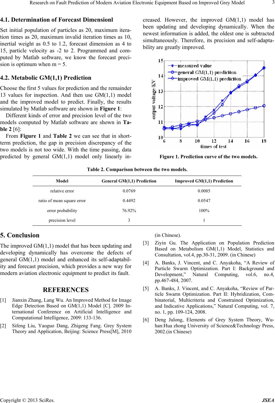

Research on Fault Prediction of Modern Aviation Electronic Equipment Based on Improved Grey Model
3
4.1. Determination of Forecast Dimensionl
Set initial population of particles as 20, maximum itera-
tion times as 20, maximum invalid iteration times as 10,
inertial weight as 0.5 to 1.2, forecast dimension as 4 to
15, particle velocity as -2 to 2. Programmed and com-
puted by Matlab software, we know the forecast preci-
sion is optimum when m = 5.
4.2. Metabolic GM(1,1) Prediction
Choose the first 5 values fo r prediction and the remainder
13 values for inspection. And then use GM(1,1) model
and the improved model to predict. Finally, the results
simulated by Matlab software are shown in Figure 1:
Different kinds of error and precision level of the two
models computed by Matlab software are shown in Ta-
ble 2 [6]:
From Figure 1 and Table 2 we can see that in short-
term prediction, the gap in precision discrepancy of the
two models is not too wide. With the time passing, data
predicted by general GM(1,1) model only linearly in-
creased. However, the improved GM(1,1) model has
been updating and developing dynamically. When the
newest information is added, the oldest one is subtracted
simultaneously. Therefore, its precision and self-adapta-
bility are greatly improved.
Figure 1. Prediction curve of the two models.
Table 2. Comparison between the two models.
Model General GM(1,1) Predic tio n Improved GM(1,1 ) Predictio n
relative error 0.0769 0.0085
ratio of mean square e rror 0.4492 0.0547
error probability 76.92% 100%
precision level 3 1
5. Conclusion
The improved GM(1,1) model that has been updating and
developing dynamically has overcome the defects of
general GM(1,1) model and enhanced its self-adaptabil-
ity and forecast precision, which provides a new way for
modern aviation electron ic equipment to predict its fault.
REFERENCES
[1] Jianxin Zhang, Lang Wu. An Improved Method for Image
Edge Detection Based on GM(1,1) Model [C]. 2009 In-
ternational Conference on Artificial Intelligence and
Computational Intelligence, 2009: 133-136.
[2] Sifeng Liu, Yaoguo Dang, Zhigeng Fang. Grey System
Theory and Application, Beijing: Science Press[M], 2010
(in Chinese).
[3] Ziyin Gu. The Application on Population Prediction
Based on Metabolism GM(1,1) Model, Statistics and
Consultation, vol.4, pp.30-31, 2009. (in Chinese)
[4] A. Banks, J. Vincent, and C. Anyakoha, “A Review of
Particle Swarm Optimization. Part I: Background and
Development,” Natural Computing, vol.6, no.4,
pp.467-484, 2007.
[5] A. Banks, J. Vincent, and C. Anyakoha, “Review of Par-
ticle Swarm Optimization. Part II: Hybridization, Com-
binatorial, Multicriteria and Constrained Optimization,
and Indicative Applications,” Natural Computing, vol. 7,
no. 1, pp. 109-124, 2008.
[6] Deng Julong, Elements of Grey System Tbeory, Wu-
han:Hua zhong University of Science&Technology Press,
2002.(in Chinese)