Applied Mathematics, 2010, 1, 316-325
doi:10.4236/am.2010.14042 Published Online October 2010 (http://www.SciRP.org/journal/am)
Using Differential Evolution Method to Solve
Crew Rostering Problem
Budi Santosa, Andiek Sunarto, Arief Rahman
Indusrial Engineering, Institut Teknologi Sepuluh Nopember,Kampus ITS Sukolilo Surabaya, Indonesia
Received April 19, 2010; revised August 24, 2010; accepted August 27, 2010
Abstract
Airline crew rostering is the assignment problem of crew members to planned rotations/pairings for certain
month. Airline companies have the monthly task of constructing personalized monthly schedules (roster) for
crew members. This problem became more complex and difficult while the aspirations/criterias to assess the
quality of roster grew and the constraints increased excessively. This paper proposed the differential
evolution (DE) method to solve the airline rostering problem. Different from the common DE, this paper
presented random swap as mutation operator. The DE algorithm is proven to be able to find the near optimal
solution accurately for the optimization problem. Through numerical experiments with some real datasets,
DE showed more competitive results than two other methods, column generation and MOSI (the one used by
the Airline). DE produced good results for small and medium datasets, but it still showed reasonable results
for large dataset. For large crew rostering problem, we proposed decomposition procedure to solve it in more
efficient manner using DE.
Keywords: Differential Evolution, Crew Scheduling, Pairing, Rostering
1. Introduction
Development of crews rostering plan which be able to
produce the high utility of crews become the priority in
human resources department in airline industry. It is
estimated that the use of optimization software for airline
could save more than US $20 million per year [1].
Saving 1% in crew utilization can save cost largerly.
Though airline crews scheduling became attention in
many operation research literature such as [1-7] but air-
line crews scheduling remains to become the main atten-
tion for many researchers due to its level of complexity
and difficulty to solve. Therefore, methods and approa-
ches which are used to solve it are continuously develo-
ped to get better result both in optimality side and speed
of computational time. Generally, solving airline crew
scheduling is done by decomposition approach [8-10]), it
devides problem into crew pairing and crew rostering.
Crew pairing is done to get initial feasible solution, that
is sequence of flight which begin and end at the same
home base. Crew rostering assigns pairings which were
arranged for the certain month to set of crews based on
individual calender.
Decomposition approach is very effective to solve the
difficult and complex problem but this method loss the
global treatment since crew pairing and crew rostering
done separately. Some other researchers developed the
integrated approach to overcome obstacle, such as Souai
and Thegem [5], where crew pairing and rostering were
done simultantly to get a better optimality level.
Many optimization methods have been developed to
solve crew scheduling to increase roster quality and to
improve computational time such as simulated annealing
[11], genetic algorithm [5], tree search algorithm [12],
hybrid genetic algorithm [13] and GASA hybrid algori-
thm [14].
This research focused on developing differential evo-
lution algorithm applied on intelligent airline crew ros-
tering system. This paper is organized as follows. The
second section reviews differential evolution (DE). Sec-
tion 3 describes the problem statement. In Section 4, we
describe our methodology. Section 5 explaines the ex-
perimental setting and the results. Section 6 concludes
the results.
2. Differential Evolution
Differential evolution is an evolutionary population-based

B. SANTOSA ET AL. 317
algorithm proposed by Storn and Price [15,16]. Since its
initiation in 1995, DE has shown its performance as a
very effective global optimizer. DE originated with Ge-
netic Annealing (GA) Algorithm. Since GA was very
slow and effective control parameters were hard to de-
termine, the modification of the GA algorithm were made.
DE uses a floating-point instead of bit-string encoding
and arithmatic operations instead of logical ones. DE
differs significantly from the evolutionary algorithms in
the sense that distance and direction information from
the current population is used to guide the search proc-
ess. DE uses the differences between two randomly cho-
sen vectors (individuals) as the base to form a third vec-
tor (individual), referred to as the target vector. Trial
solutions are generated by adding weighted difference
vectors to the target vector. This process is referred to as
the mutation operator where the target vector is mutated.
The next step is recombination or crossover which is
applied to produce an offspring. This new individual is
accepted only if it improves on the fitness of the parent
individual. The basic DE algorithm is described in more
detail below [16].
2.1. Initialization
In this step, a set of initial solutions are genereted rando-
mly. A random number generator assigns each variable
of each vector value from within specified range, lower
bound, bL, and upper bound, bU. For example the initial
value (g = 0) of the jth variable of ith vector is:



,,, ,,
rand0,1 .
j

0
xbbb
j
ijUjLjL
(1)
where, randj (0,1), returns a uniformly distributed random
number from within the range [0,1].
2.2. Mutation
DE mutates and recombines the population to produce a
population of N-trial vectors. In particular, differential
mutation adds a scaled, randomly sampled, vector dif-
rence of third vector. To combine three different ran-
mly chosen vectors to create the mutant vector, vi,g, the
following equation is used:


,,,
+.
, 012
vxFx x
igrgr grg (2)
where the scale factor, F (0, 1+) is a positive real
number that control the rate at which the population
evolve. The vector index, r0, r1, and r2, can be chosen
randomly and meet r0  r1  r2  i.
2.3. Crossover
DE employs the uniformly crossover. Crossover builds
trial vectors out of parameter value that have been copied
from two different vectors. In particular, DE crosses each
vector with a mutant vector to creat ui,g.
,,
,,,
,,
,((0,1) ,max
,
j
vifrand Crorjj
xotherwise







jig
ig jig
jig
uu
(3)
The crosover probability, Cr ∊ [0,1], is user-defined
value that controls the fraction of parameter value that
are copied from the mutant.
2.4. Selection
If the trial vector, ui,g, has an equal or lower objective
function value (better fitness value) than that of its target
vector, xi,g, it replaces the target vector in the next
generation; otherwise, the target retains its place in the
population at least one more generation.
,,,
,1
,
,()()
,
ig ig
iff ufx
otherwise







ig
ig ig
u
xx (4)
Once the new population created, the process of
mutation, recombination, and selection are repeated until
the optimum solution is achieved or prespesified termina--
tion criterion is satisfied, e.g., the number of generations
reaches preset maximum, gmax.
DE has been applied in many field successfully. In
1995, DE has been used by Ken to solve 5-dimension
Chebyshev model. By the time, Ken modified genetic
annealing algorithm with differential mutation operator.
Different from genetic annealing, DE has not found
some difficulty to find the coefficient even 33-dimension
Chebyshev.
Tasgetiren [15] used a discrete differential evolution
(DDE) algorithm to solve the single machine total earli-
ss and tardiness penalties with a common due date. A
new binary swap mutation operator called Bswap is pre-
nted. In addition, the DDE algorithm is hybridized with a
local search algorithm to further improve the perform-
ance of the DDE algorithm. The performance of the
proposed DDE algorithm is tested on 280 benchmark in-
stances ranging from 10 to 1000 jobs from the OR Li-
brary. The computational experiments showed that the
proposed DDE algorithm has generated better results
than those in the literature in terms of both solution qual-
ity and computational time.
A genetic differential evolution (GDE) was derived
from the differential evolution (DE) and incorporated
with the genetic reproduction mechanisms, namely cross-
over and mutation used to solve traveling salesman pro-
blems (TSP). The Greedy Subtour Crossover (GSX) was
employed to generate an offspring to denote the differ-
ence of the parents. A modified ordered crossover (MOX)

B. SANTOSA ET AL. 318
was employed to perform mutation to generate trial vec-
tor with a user defined parameter, the parameter were
used to control the rates of the target vector components
and the mutated vector components in the trial vector.
Moreover, a 2-opt local search was implemented to en-
hance local search performance. GDE was implemented
to the well-known TSP with 52, 100 and 200 cities with
variable parameters. Based on analysis and discussion on
the results, typical values of the parameters were given,
with which GDE provided effective and robust perform-
ance [18].
Omran and Salman [19] improved Differential evolu-
tion by combining with chaotic search, opposition-based
learning, and quantum mechanics, called CODEQ, to
solve constrained optimization problems. The perform-
ance of the proposed approach when applied to five con-
strained benchmark problems is investigated and com-
pared with other approaches proposed in the literature.
The experiments conducted show that CODEQ provides
excellent results with the added advantage of no parame-
ter tuning.
3. Problem Statement
There are two main processes in the airline crew plan-
ning. These two process are pairing and rostering. Pair-
ing, is the step where the flying activities are created.
The flight timetable is used as input to form sequences of
flights, known as pairings. The timetable horizon usually
covers a period of 4-6 weeks. The main objective of this
process is to utilize the minimum number of crew to
cover the complete timetable. Rostering is the step where
the created pairings are assigned to actual crew (pilot and
stewardess), with regard to the qualifications and previ-
ously assigned activities, referred to as pre-assignments,
of the crew. The objective is to find feasible assignments
that minimize costs and match the notion of quality of
life for the crew imposed by the airline [9]. In this
context, problem of airline crew scheduling generally
varies among different countries. Especially in rostering
problem since each country may impose different set of
regulations, rules and policies. The speed of roster
construction is a critical matter in airline crew schedule-
ing. In [9], it is stated that for monthly planning, solution
should be obtained within 15-20 minutes. While, for
shorter horizon planning, such as daily planning, where
there are some changes to roster, solutions should be
obtained within 1-5 minutes. Therefore, solving optimi-
zation problem of airline crew scheduling in time manner
become very important.
In this paper two main problems are addressed. First,
how to mathematically formulate the problem of airline
crew scheduling. This formulation includes the construc-
tion of objective function and spesific set of constraints
which influence the roster quality. We modified the
model which is developed by Lučić and Teodorović [11]
based on the real condition of rostering in the airline
under study. We modified the single crew and single
aircraft scheduling model becomes multiple crews and
multiple aircrafts model. We also added open time crite-
ria to the objective function. Second, how to solve the
model using differential evolution approach with consi-
dering the simplicity of the model, quality of the resulting
roster, and computational time.
3.1. Index
k is index for kind of crews k = 1,,K. For example, k =
1 is for Pilot F-100; k = 2 is for Pilot CN-235; and k = 8
is for stewardess and etc.
i is index for numbers of crew members (1,,mk). For
example m
5 = 17 is the number of crew members for
Boeing 737-200, and m8 = 55 is the number of stewardess
of Boeing 737-200.
j is index rotation/pairing which assigned to crew
members (1,,nk). For example n5 = 82, is the number
of pairings for Being 737-200.
l is number of days in a month (1,,31).
3.2. Parameters
djk is length of rotation-j which assigned to crew k. (in
hours).
1,ifmember from crew can be assigned to day
0, otherwise
ilk
i kl
p 

1,if/ assigned to crew start to day
0, otherwise
jlk
rotationpairing j kl
q 

dmax,k is maximum flight times crew k for one month;
vjk is numbers of take-off rotation j assigned to crew k;
vmax,k is maximum take-off in one month;
Dmin,jk is minimum of numbers of crews k needed to
complete rotation j;
tjk is numbers of duty period needed by crew k to com-
plete rotation j;
tmax,k is maximum of flying day before free day.
1,if rotationoverlap with rotation when assigned to crew
0, otherwise
rsk
rsk
n 



B. SANTOSA ET AL. 319
3.3. Objectives Function
The objective function of this airline crew rostering is
minimizing three terms of criterias.
Cost of roster
Cost of roster paid by the airline company to crew is
variable cost. By assumption that salary per hour is same
to all crew, cost of roster can be represented by actual
flying hours.
11
min1,,
kk
mn
jk ijk
ij
dx kK


  (5)
Deviation of flying days between crew members
Let k t be the average flying days per month for crew
member k, then
11 1,,
kk
mn
jk ijk
ij
k
k
tx
tkK
m



 (6)
The deviation of total flying days per month can be
formulated as
11
min 1,,
kk p
mn
k
jk ijk
ij
tx tkK


  (7)
where p is positive integer. In this paper we use p = 1.
Open time
Open time is days when a crew member does not have
flying duty. If there are 31 days in a scheduling month,
then open time for crew member k can be formulated as
11
min31 1,,
kk
mn
jk ijk
ij
tx kK





  (8)
3.4. Constraints
There are some constraints which must be satisfied
when constructing a roster. The following are the const-
raints used:
Flight time constraint
Maximum flying hours for pilot and co-pilot is 110
hours per month, and for cabin crew is 120 hours per
month. So dmax,k = 110 for k = 1,,7 and dmax,k = 120 for
k = 8.
max,
1
1,...,, 1,,
k
n
jk ijkkk
j
dxdim kK

 
 (9)
Duty period constraint
Maximum duty period allowed to crew member k is 21
days.
1
21 1,,, 1,,
k
n
jk ijkk
j
txim kK

 
 (10)
Numbers of take-off
Numbers of maximum take off allowed to pilot is 90,
then vmax,k = 90. But, cabin crew have no take off con-
straint.
max,
1
1,,, 1,,
k
n
jk ijkkk
j
vxvim kK

 
 (11)
Numbers of crew reqirement
Every rotation needs minimum numbers of crew.
min,
1
1,,, 1,,
k
m
ijk jkk
i
x
Dj nkK

 
 (12)
Free day constraint
Every crew member must be given free days after 7
flying days.
7
1
7 1,,, 1,,23, 1,,8
k
np
jk ijkjklk
jlp
txqim pk


 
 
(13)
Rotation without free day
When crew members complete this rotation not al-
lowed to have free day.
1
31
111
1,,, 1,,
jk
kk lt
nn
ijkijk jkliskk
jjl sl
x
xqpi mkK

 

 
(14)
No overlap constraint
Two rotations in series may not be overlap each other.
It means that precedence rotation must be finished when
following rotation will start.
1
()0
1,,, 1,,, 1,,
k
n
ijkjsk isk
s
kk
xxsj
imjnkK






(15)
Airline rostering problem is optimization problem with
many constraints. It falls to constrained optimiza-
tion problem. To use DE to solve this original problem we have
to transform the problem into an unconstrained optimiza-
tion problem. We use external penalty function method
[20,21] to do this transformation. Basically, this method
incurs big penalty while the solution violated any con-
straints. The resulting constrained optimization problem
is as follows


12
111 1
3 11223344
11
55 6677 88
min
31
kkk k
kk
p
mnm n
k
jk ijkjk ijk
iji j
mn
jk ijk
ij
dxtx t
t xrCrCrCrC
rC rCrCrC


 



 



 
 (16)
where:
2
1max,
11
max0, 1,,
kk
mn
jk ijkk
ij
CdxdkK









 

B. SANTOSA ET AL. 320
2
2max,
11
max0, 1,,
kk
mn
jk ijkk
ij
CvxvkK









 
2
3min,
11
max0, 1,,
kk
nm
ijk jk
ji
CxDkK









 
2
7
4
11
max0,7 1,,
kk
mn p
jk ijkjkl
ijlp
CtxqkK










 
2
1
31
5
1111
max0,
1,,
jk
kkk
lt
mnn
ijkijk jklisk
ijjl sl
Cxxqp
kK

 










 

2
1
31
6
1111
min0,
1,,
jk
kkk
lt
mnn
ijkijk jklisk
ijjl sl
Cxxqp
kK

 


  






 

2
7
11
max0,() 1,,
kk
mn
ijkjsk isk
is
CxxsjkK 









 
2
8
11 1
min0,() 1,,
kk k
mn n
ijkjsk isk
ij s
CxxsjkK 
 


 





 
where β1, β2, and β3 are weight coeficients of the objec-
tive function, r1,…,r8 are penalties which are given since
model violate any constraints where r1,…,r8 → ∞ will
assure that algorithm will satisfy constraint early before
considering objective function. Equation (16) becomes
the fitness function of DE method. If we assume cost of
roster more important than cost of deviation of flying day
and more important than open time, then β1, β2, and β3
are selected carefully where β1  β2  β3 and assure
followed inequality is true :
12
111 1
3
11
31
kkkk
kk
p
mnm n
k
jk ijkjk ijk
iji j
mn
jk ijk
ij
dxtxt
tx


 






 



(17)
Term (17) will assure hirarchical ordering of solving
iteratively by DE.
4. Solving the Model Using DE
In this paper we applied this model on a real case taken
from MNA (Merpati Nusantara Airlines), Ltd., a private
airline company based in Indonesia [22,23]. To solve the
above problem we pursue the following steps of DE.
4.1. Initialization
Initial solution xijk is defined by generating n_pop binary
random numbers (0 or 1) of dimension nk × mk. Let Xnp,0
be the initial solution population np, then
,0 [0;1] 1..., np np
X
randnpn pop

 (18)
Randnp[0;1] is binary random 0 or 1 of population np.
4.2. Mutation
Different from those which usually used as a mutation
operator in DE as indicated in Equation (2), this paper
introduce a random swap as a mutation operator. Let r0
be random number between 0 and 1 with nk × mk dimen-
sion for each population np, and vnp,r0,g be element of
solution V at column r0 at generation g. If Wnp,g-1 is the
best population for generation g-1 and wnp,r0,g-1 is the
element at column r0 of Wnp,g-1, then mutant of generation
g is defined as
,0, 10
,0,
,0, 1
(1) mod(2),if
,otherwise
np rgm
np rg
np rg
Wrc
vW








(19)
where cm is mutation probability (0 < cm <1) which
represents mutation power imposed to the best popula-
tion of previous generation. Term Wnp,r0,g-1 mod(2) means
what value left after dividing Wnp,r0,g-1 by 2. The selection
of cm must be done carefully because too small cm can
cause old solution is difficult to exit from local optimum.
While, too big cm causes noise solution such that fast
convergence toward global optima can not be achieved.
Selecting cm accurately becomes the successful key of
implementing this algorithm.
As an illustration how this mutation operator works,
notice the following example. Suppose we have 3 pilots
and 4 pairings, use cm = 0.2.
Suppose we have W0 (current solution):
0
1000
11 1 1
1010
W











Entry (i,j) = 1 indicates a pilot i be placed in pairing j,
entry(i,j) = 0, otherwise. After generating randomly,
suppose we got:
0
0,100, 400, 080,70
0,30 0,20 0,90 0,15
0,850,05 0,25 0,55
r











To have a new solution, apply Equation (19). By
comparing r0 and cm for each corresponding entry in W0
and r0, we have matrix W’0 , where each entry (typed in
bold) should be changed since r0 < cm.
0
1000
' 1111
1010
W












B. SANTOSA ET AL. 321
The changes should be made as follows
Cell(1,1) v = (w0 + 1) mod(2) = (1 + 1) mod(2) = 2
mod(2) = 0
Cell(1,3) v = (w0 + 1) mod(2) = (0 + 1) mod(2) = 1
mod(2) = 1
Cell(2,4) v = (w0 + 1) mod(2) = (1 + 1) mod(2) = 2
mod(2) = 0
Cell(3,2) v = (w0 + 1) mod(2) = (0 + 1) mod(2) = 1
mod(2) = 1
The other entries of W0 remains the same as ro ≥ cm,.
Therefore, we obtain the new solution
0010
1110
1110
V





We follow this process each time the algorithm is on the
mutation step.
4.3. Crossover
Crossover changes over parent solution Xnp,g by mutant
solution Vnp,g to construct a new solution Unp,g. Cross-
over is done by defining threshold probability (0 < cr <
1) for mutant to change current solution. Then we gener-
ate n_pop random numbers (0,1). If the random number
< cr, then the mutant replaces the current solution and
otherwise.
,
,
,
,(0,1)
,
np gnpr
np g
np g
Vif randc
UXotherwise





 (20)
4.4. Selection
This process is done by comparing the fitnesses of the
parent solution and the new solution which is produced
from crossover process. The new population will replace
the old population only if the new population has better
fitness than that of the old population. The fitness func-
tion refers to Equation (16). Then, the solution of the
next generation Xnp,g+1 can be obtained from this for-
mula:
,, ,
,1
,
,( )()
,
np gnp gnp g
np g
np g
UiffU fX
XXotherwise






 (21)
where f(Unp,g) and f(Xnp,g) are the fitness of Unp,g and Xnp,g
respectively.
The constructed mathematical model consists of some
aspirations/criterias as the objective function and some
constraints. The objective function includes minimum
flying times, deviation of flying days, and open time.
Some constraints which are considered when construc-
ting a roster include overlap, crew requirement of pairing,
free days before seven days of flying days, maximum
flying times, and maximum numbers of take off.
5. Experiments and Analysis
We used Matlab to implement DE algorithm. The expe-
riments were done using the datasets shown in Table 1.
The datasets consist of pairings, numbers of crews, type
of fleed and rules. Datasets are divided into two catego-
ries: small and large datasets. Small dataset consists of
assignment of F-100, CN-235, DHC-6, and Cassa 212
pilot. While, large dataset consists of assignment of
Boeing 737-200 pilot and stewardess.
The experiments aim to assign crew members in which
pairings. The results of the experiments on small datasets
were compared with column generation [22,23] and
MOSI (method used by the company). For large datasets
we included exact decomposition as a comparative method
[23].
Probability of mutation (cm) and probability of cross-
er (cr) are the key succes factors for DE implementation.
Therefore, these two parameters should be determined
carefully. The precise parameter values will lead to the
global optimal solution. In this paper, these parameters
settings were done through trial process. The best cm, is
determined by using one dataset (Cassa 212) with npop =
50, gmax = 50, cr = 0.7 and the experiments were done
with 5 replications. Table 2 shows the objective function
values for different cm. The best value is typed in bold.
We found that cm = 0.05 is the best one.
Using cm = 0.05, the same procedure was done to find
the best cr. The results are shown in Table 3.
Next, using combination of cm and cr we tried to
determine the best values of these two parameters.
Through experiments, we obtained the best combination
between cm and cr are 0.1 and 0.5 as shown in bold in
Table 4.
Criteria in the objective function are weighted based
on their significances. In this paper we put roster cost
minimization as the most significance followed by devia-
tion of minimum flying days and open time with weights
of 104, 102 and 1 respectively. Other parameter needs to
set up is pinalty for the constraints. Penalties for overlap
and rotation without free day, number of pilot require-
ments and day off constraints are 1015, 1013 and 1011 res-
pectively based on their signifances.While, the penalties
for flying day, flying times, and numbers of take off are
set to 106 as these constraints are assumed to be the same
important.
Experimental results for small datasets are indicated in
Table 5. For the flying time criterion, DE spent more

B. SANTOSA ET AL. 322
Table 1. Characteristic of the datasets.
No Name of aircraft Type of crews Numbers
of crews
Numbers of
pairings
1 F-100 Pilot 5 4
2 CN-235 Pilot 4 8
3 DHC-6 Pilot 3 10
4 Cassa-212 Pilot 6 13
5 Boeing 737-200 Pilot 17 82
6 Boeing 737-200 stewardess55 114
Table 2. Average objective function values on different cm.
No cm Average objective function value
(× 1013)
1 0.000 9,980
2 0.025 41.00
3 0.050 3.00
4 0.075 22.60
5 0.100 7.60
6 0.125 48.20
7 0.150 122.20
8 0.175 140.80
9 0.200 163.40
Table 3. Average objective function values on different cr.
No cr Average objective function value
(× 1013)
1 0.300 22.00
2 0.350 43.20
3 0.400 21.80
4 0.450 80.60
5 0.500 42.60
6 0.550 41.00
7 0.600 22.60
8 0.650 40.60
9 0.700 23.40
time than two other methods. The reason is because DE
did not violate pilot requirement constraint. This is
different with column generation and MOSI which
violated pilot requirement constraint. It shows that DE,
column generation, and MOSI produced the same per-
formance to meet the roster constraints. Except for Cassa
212, DE can meet all of the constraints. While, column
generation and MOSI violate pilot requirements con-
straints. Column generation and MOSI just assign 1 out
of 2 required pilots to pairing 8981. From roster quality
side, DE is only inferior for flying times criterion for
Cassa 212 aircraft. The other methods show the same
results for other assignments.
Table 6 shows the total deviation of average flying
days for three methods. We see that DE is superior for all
assignments except for Cassa 212. This proves that DE
produced good roster quality. From Table 6, we see that
DE produced better deviation of flying days than other
methods for three assignments and MOSI is superior for
Cassa 212.
Table 4. Average objective function values on different com-
bination of cm and cr.
No cm c
r Average objective
function value (× 1013)
1 0.05 0.400 21.80
2 0.05 0.5 42.60
3 0.05 0.6 22.60
4 0.05 0.7 3.00
5 0.1 0.4 22.20
6 0.1 0.5 2.40
7 0.1 0.6 23.20
8 0.1 0.7 7.60
Tabel 5. Comparison of flying time.
Fying time
Name of
Aircraft DE Column Generation MOSI
F-100 66.0 66.0 66.0
CN-235 92.0 92.0 92.0
DHC-6 156.0 156.0 156.0
Cassa 212 251.0 242.0 242.0
Tabel 6. Comparison of deviation of flying days.
Fying time
Name of
Aircraft DE Column Generation MOSI
F-100 7.2 14.4 14.4
CN-235 2.0 12.0 4.0
DHC-6 8.0 10.7 11.3
Cassa 212 11.3 21.0 6.0

B. SANTOSA ET AL. 323
For the open time criteria, as shown in Table 7, DE
produced superior results compared to the other methods
for Cassa 212 and the same results for other assignments.
Dataset of pilots and stewardess assignment on Boeing
737-200 aircraft has a larger size. This dataset consists of
17 pilots with 82 pairings and 55 stewardess with 114
pairings. It required high number of iterations and com-
putational time to obtain near optimal solution if random
initial solutions were used. We proposed a sequence of
partial optimization and total optimization techniques. In
partial optimization, the dataset is splitted into several
smaller sets and the corresponding optimization problems
were solved by DE method. At the end of this stage, all
of solutions were combined all together to form initial
solution for the total optimization problem. Setting the
initial solution through this process decreased the compu-
tational time significantly.
For the pilot assignment of Boeing 737-200, number
of pairings is much higher than the available pilots.
Therefore the resulting flight schedules violate several
constraints. The results for this assignment are shown in
Table 8. The table presents the flying days and the actual
difference produced by each pilot. In this case, we com-
pared 6 methods namely differential evolution (DE), col-
umn generation, MOSI, exact decomposition with 21
flying days (DEC21), exact decomposition with 20 fly-
ing days (DEC20) and exact decomposition with 19 fly-
ing days (DEC19). The results are presented in Table 8.
Table 7. Comparison of open time.
Open time
Name of
Aircraft DE Column Generation* MOSI*
F-100 137.0 137.0 137.0
CN-235 88.0 88.0 88.0
DHC-6 50.0 50.0 50.0
Cassa 212119.0 123.0 123.0
Table 8. Comparison flying days and differences.
Differential
Evolution
Column
Generation* MOSI* Method DEC21**
Method
Dec20
Method
Dec19
Pilot flying
day diff. flying day diff. flying day diff. flying day diff. Fying days diff Fying daya diff
1 21 0 20 0 21 0 20 0 21 0 22 1
2 20 0 18 0 21 0 22 1 23 2 22 1
3 20 0 20 0 23 2 26 5 23 2 24 3
4 21 0 20 0 22 1 24 3 23 2 23 2
5 21 0 17 0 18 0 17 0 18 0 17 0
6 21 0 20 0 22 1 24 3 23 2 23 2
7 22 1 21 0 16 0 18 0 17 0 20 0
8 21 0 26 5 21 0 22 1 24 3 22 1
9 20 0 16 0 17 0 20 0 18 0 19 0
10 18 0 18 0 16 0 13 0 16 0 14 0
11 22 1 23 2 22 1 19 0 19 0 19 0
12 21 0 21 0 21 0 22 1 22 1 21 0
13 20 0 24 3 24 3 22 1 21 0 20 0
14 21 0 23 2 24 3 20 0 20 0 22 1
15 20 0 20 0 19 0 21 0 21 0 21 0
16 20 0 22 1 21 0 21 0 21 0 22 1
17 22 1 22 1 23 2 18 0 18 0 17 0
Total 351 3 351 14 351 13 349 15 348 12 348 12
Avg
Std.D
20.65
0.99 20.65 2.57 20.65 2.57 20.53 3.04 20.47 2.43 20.47 2.40
Number of pilot
violate flying.
days
3 6 7 7 8 8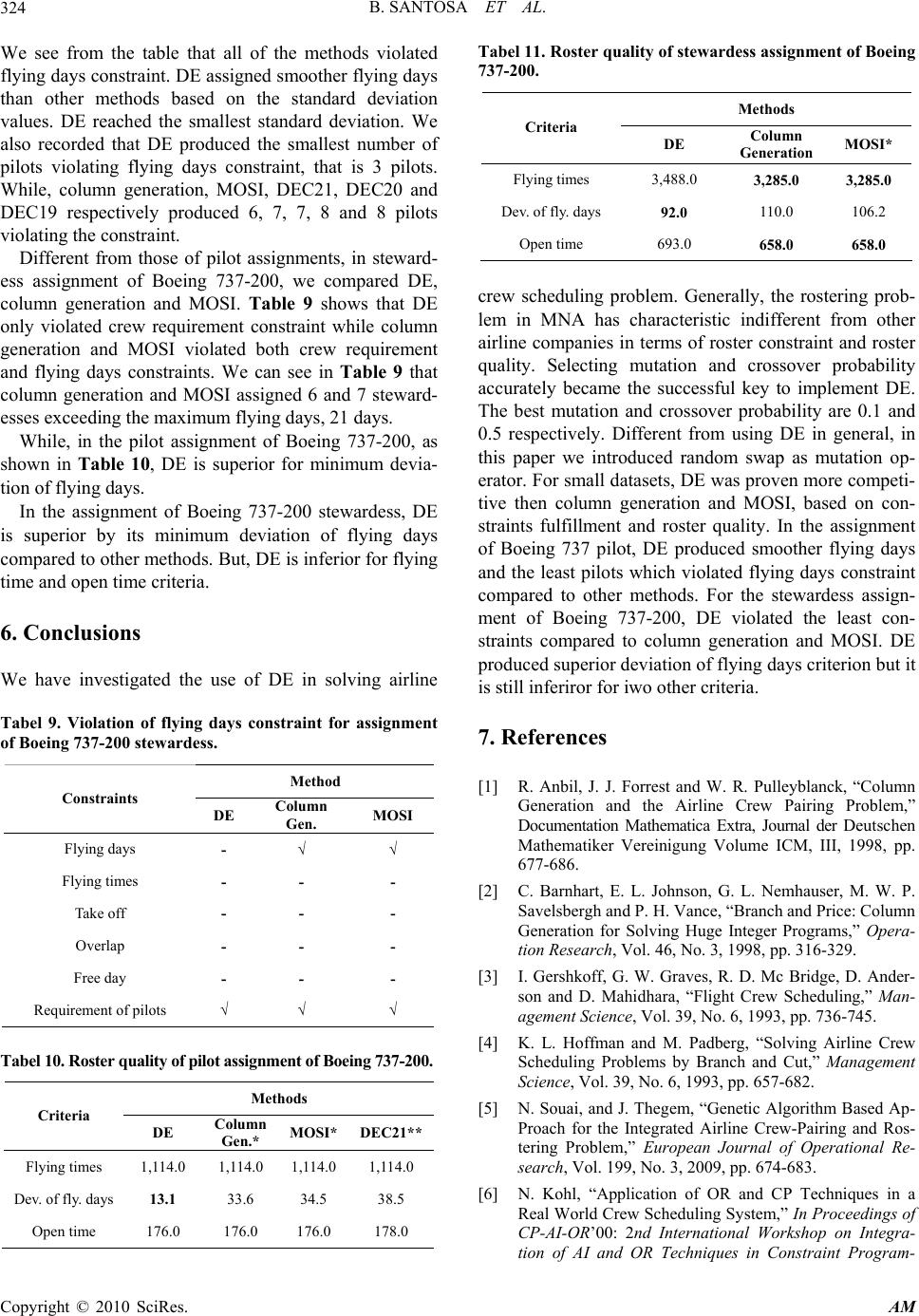

B. SANTOSA ET AL. 324
We see from the table that all of the methods violated
flying days constraint. DE assigned smoother flying days
than other methods based on the standard deviation
values. DE reached the smallest standard deviation. We
also recorded that DE produced the smallest number of
pilots violating flying days constraint, that is 3 pilots.
While, column generation, MOSI, DEC21, DEC20 and
DEC19 respectively produced 6, 7, 7, 8 and 8 pilots
violating the constraint.
Different from those of pilot assignments, in steward-
ess assignment of Boeing 737-200, we compared DE,
column generation and MOSI. Table 9 shows that DE
only violated crew requirement constraint while column
generation and MOSI violated both crew requirement
and flying days constraints. We can see in Table 9 that
column generation and MOSI assigned 6 and 7 steward-
esses exceeding the maximum flying days, 21 days.
While, in the pilot assignment of Boeing 737-200, as
shown in Table 10, DE is superior for minimum devia-
tion of flying days.
In the assignment of Boeing 737-200 stewardess, DE
is superior by its minimum deviation of flying days
compared to other methods. But, DE is inferior for flying
time and open time criteria.
6. Conclusions
We have investigated the use of DE in solving airline
Tabel 9. Violation of flying days constraint for assignment
of Boeing 737-200 stewardess.
Method
Constraints
DE Column
Gen. MOSI
Flying days - √ √
Flying times - - -
Take off - - -
Overlap - - -
Free day - - -
Requirement of pilots √ √ √
Tabel 10. Roster quality of pilot assignment of Boeing 737-200.
Methods
Criteria
DE Column
Gen.* MOSI* DEC21**
Flying times 1,114.0 1,114.0 1,114.0 1,114.0
Dev. of fly. days 13.1 33.6 34.5 38.5
Open time 176.0 176.0 176.0 178.0
Tabel 11. Roster quality of stewardess assignment of Boeing
737-200.
Methods
Criteria
DE Column
Generation MOSI*
Flying times 3,488.0 3,285.0 3,285.0
Dev. of fly. days 92.0 110.0 106.2
Open time 693.0 658.0 658.0
crew scheduling problem. Generally, the rostering prob-
lem in MNA has characteristic indifferent from other
airline companies in terms of roster constraint and roster
quality. Selecting mutation and crossover probability
accurately became the successful key to implement DE.
The best mutation and crossover probability are 0.1 and
0.5 respectively. Different from using DE in general, in
this paper we introduced random swap as mutation op-
erator. For small datasets, DE was proven more competi-
tive then column generation and MOSI, based on con-
straints fulfillment and roster quality. In the assignment
of Boeing 737 pilot, DE produced smoother flying days
and the least pilots which violated flying days constraint
compared to other methods. For the stewardess assign-
ment of Boeing 737-200, DE violated the least con-
straints compared to column generation and MOSI. DE
produced superior deviation of flying days criterion but it
is still inferiror for iwo other criteria.
7. References
[1] R. Anbil, J. J. Forrest and W. R. Pulleyblanck, “Column
Generation and the Airline Crew Pairing Problem,”
Documentation Mathematica Extra, Journal der Deutschen
Mathematiker Vereinigung Volume ICM, III, 1998, pp.
677-686.
[2] C. Barnhart, E. L. Johnson, G. L. Nemhauser, M. W. P.
Savelsbergh and P. H. Vance, “Branch and Price: Column
Generation for Solving Huge Integer Programs,” Opera-
tion Research, Vol. 46, No. 3, 1998, pp. 316-329.
[3] I. Gershkoff, G. W. Graves, R. D. Mc Bridge, D. Ander-
son and D. Mahidhara, “Flight Crew Scheduling,” Man-
agement Science, Vol. 39, No. 6, 1993, pp. 736-745.
[4] K. L. Hoffman and M. Padberg, “Solving Airline Crew
Scheduling Problems by Branch and Cut,” Management
Science, Vol. 39, No. 6, 1993, pp. 657-682.
[5] N. Souai, and J. Thegem, “Genetic Algorithm Based Ap-
Proach for the Integrated Airline Crew-Pairing and Ros-
tering Problem,” European Journal of Operational Re-
search, Vol. 199, No. 3, 2009, pp. 674-683.
[6] N. Kohl, “Application of OR and CP Techniques in a
Real World Crew Scheduling System,” In Proceedings of
CP-AI-OR’00: 2nd International Workshop on Integra-
tion of AI and OR Techniques in Constraint Program-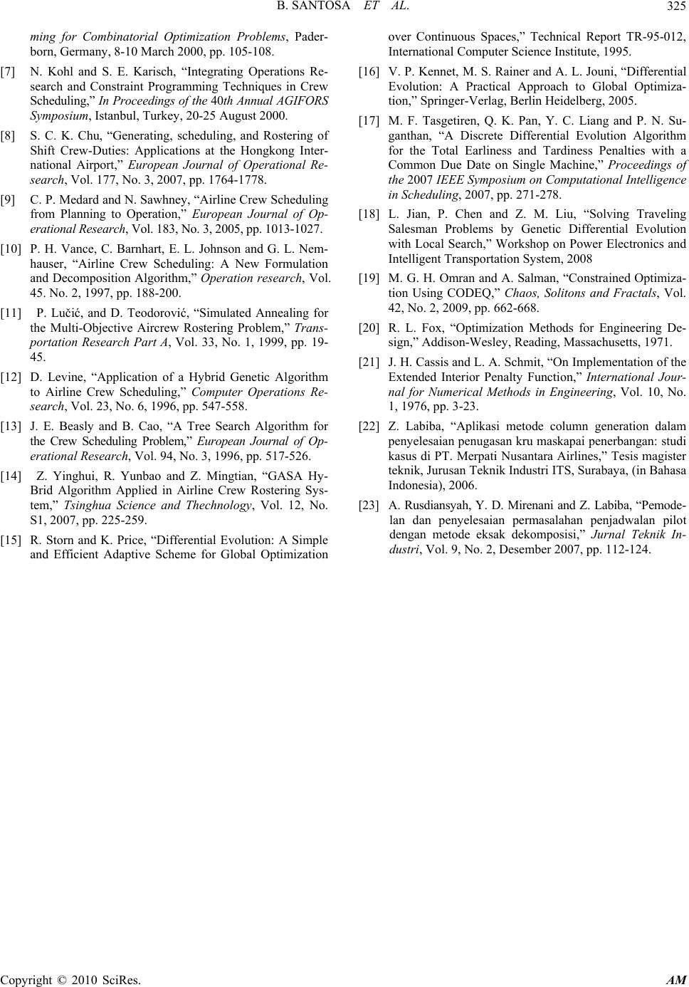

B. SANTOSA ET AL. 325
ming for Combinatorial Optimization Problems, Pader-
born, Germany, 8-10 March 2000, pp. 105-108.
[7] N. Kohl and S. E. Karisch, “Integrating Operations Re-
search and Constraint Programming Techniques in Crew
Scheduling,” In Proceedings of the 40th Annual AGIFORS
Symposium, Istanbul, Turkey, 20-25 August 2000.
[8] S. C. K. Chu, “Generating, scheduling, and Rostering of
Shift Crew-Duties: Applications at the Hongkong Inter-
national Airport,” European Journal of Operational Re-
search, Vol. 177, No. 3, 2007, pp. 1764-1778.
[9] C. P. Medard and N. Sawhney, “Airline Crew Scheduling
from Planning to Operation,” European Journal of Op-
erational Research, Vol. 183, No. 3, 2005, pp. 1013-1027.
[10] P. H. Vance, C. Barnhart, E. L. Johnson and G. L. Nem-
hauser, “Airline Crew Scheduling: A New Formulation
and Decomposition Algorithm,” Operation research, Vol.
45. No. 2, 1997, pp. 188-200.
[11] P. Lučić, and D. Teodorović, “Simulated Annealing for
the Multi-Objective Aircrew Rostering Problem,” Trans-
portation Research Part A, Vol. 33, No. 1, 1999, pp. 19-
45.
[12] D. Levine, “Application of a Hybrid Genetic Algorithm
to Airline Crew Scheduling,” Computer Operations Re-
search, Vol. 23, No. 6, 1996, pp. 547-558.
[13] J. E. Beasly and B. Cao, “A Tree Search Algorithm for
the Crew Scheduling Problem,” European Journal of Op-
erational Research, Vol. 94, No. 3, 1996, pp. 517-526.
[14] Z. Yinghui, R. Yunbao and Z. Mingtian, “GASA Hy-
Brid Algorithm Applied in Airline Crew Rostering Sys-
tem,” Tsinghua Science and Thechnology, Vol. 12, No.
S1, 2007, pp. 225-259.
[15] R. Storn and K. Price, “Differential Evolution: A Simple
and Efficient Adaptive Scheme for Global Optimization
over Continuous Spaces,” Technical Report TR-95-012,
International Computer Science Institute, 1995.
[16] V. P. Kennet, M. S. Rainer and A. L. Jouni, “Differential
Evolution: A Practical Approach to Global Optimiza-
tion,” Springer-Verlag, Berlin Heidelberg, 2005.
[17] M. F. Tasgetiren, Q. K. Pan, Y. C. Liang and P. N. Su-
ganthan, “A Discrete Differential Evolution Algorithm
for the Total Earliness and Tardiness Penalties with a
Common Due Date on Single Machine,” Proceedings of
the 2007 IEEE Symposium on Computational Intelligence
in Scheduling, 2007, pp. 271-278.
[18] L. Jian, P. Chen and Z. M. Liu, “Solving Traveling
Salesman Problems by Genetic Differential Evolution
with Local Search,” Workshop on Power Electronics and
Intelligent Transportation System, 2008
[19] M. G. H. Omran and A. Salman, “Constrained Optimiza-
tion Using CODEQ,” Chaos, Solitons and Fractals, Vol.
42, No. 2, 2009, pp. 662-668.
[20] R. L. Fox, “Optimization Methods for Engineering De-
sign,” Addison-Wesley, Reading, Massachusetts, 1971.
[21] J. H. Cassis and L. A. Schmit, “On Implementation of the
Extended Interior Penalty Function,” International Jour-
nal for Numerical Methods in Engineering, Vol. 10, No.
1, 1976, pp. 3-23.
[22] Z. Labiba, “Aplikasi metode column generation dalam
penyelesaian penugasan kru maskapai penerbangan: studi
kasus di PT. Merpati Nusantara Airlines,” Tesis magister
teknik, Jurusan Teknik Industri ITS, Surabaya, (in Bahasa
Indonesia), 2006.
[23] A. Rusdiansyah, Y. D. Mirenani and Z. Labiba, “Pemode-
lan dan penyelesaian permasalahan penjadwalan pilot
dengan metode eksak dekomposisi,” Jurnal Teknik In-
dustri, Vol. 9, No. 2, Desember 2007, pp. 112-124.