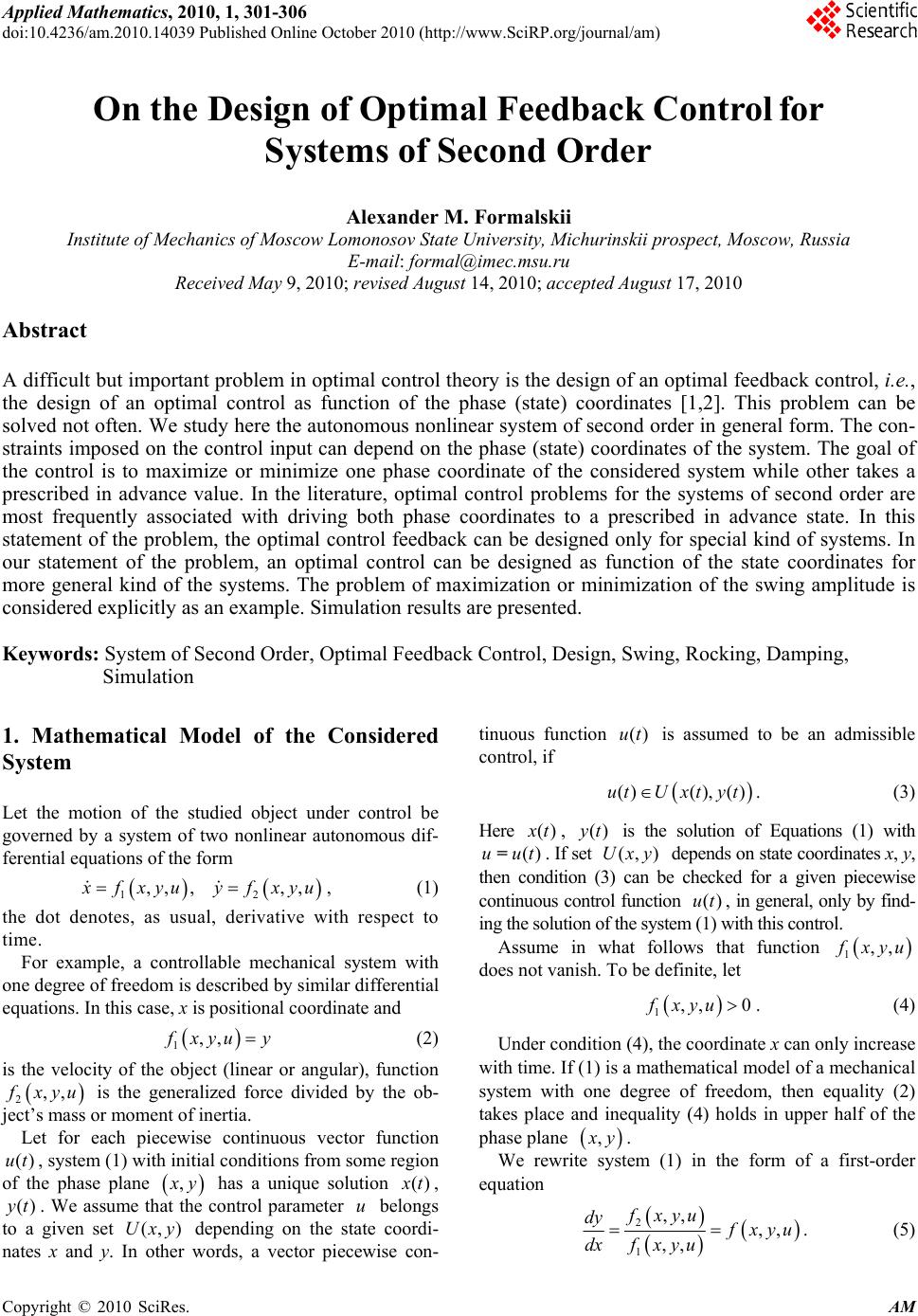Applied Mathematics, 2010, 1, 301-306
doi:10.4236/am.2010.14039 Published Online October 2010 (http://www.SciRP.org/journal/am)
On the Design of Optimal Feedback Control for
Systems of Second Order
Аlexander М. Formalskii
Institute of Mechanics of Moscow Lomonosov State University, Michurinskii prospect, Moscow, Russia
Received May 9, 2010; revised August 14, 2010; accepted August 17, 2010
Abstract
A difficult but important problem in optimal control theory is the design of an optimal feedback control, i.e.,
the design of an optimal control as function of the phase (state) coordinates [1,2]. This problem can be
solved not often. We study here the autonomous nonlinear system of second order in general form. The con-
straints imposed on the control input can depend on the phase (state) coordinates of the system. The goal of
the control is to maximize or minimize one phase coordinate of the considered system while other takes a
prescribed in advance value. In the literature, optimal control problems for the systems of second order are
most frequently associated with driving both phase coordinates to a prescribed in advance state. In this
statement of the problem, the optimal control feedback can be designed only for special kind of systems. In
our statement of the problem, an optimal control can be designed as function of the state coordinates for
more general kind of the systems. The problem of maximization or minimization of the swing amplitude is
considered explicitly as an example. Simulation results are presented.
Keywords: System of Second Order, Optimal Feedback Control, Design, Swing, Rocking, Damping,
Simulation
1. Mathematical Model of the Considered
System
Let the motion of the studied object under control be
governed by a system of two nonlinear autonomous dif-
ferential equations of the form
 
12
,, ,,,
x
fxyuyf xyu

, (1)
the dot denotes, as usual, derivative with respect to
time.
For example, a controllable mechanical system with
one degree of freedom is described by similar differential
equations. In this case, x is positional coordinate and

1,,
f
xyu y (2)
is the velocity of the object (linear or angular), function

2,,
f
xyu is the generalized force divided by the ob-
ject’s mass or moment of inertia.
Let for each piecewise continuous vector function
()ut , system (1) with initial conditions from some region
of the phase plane

,
x
y has a unique solution ()
x
t,
()yt . We assume that the control parameter u belongs
to a given set (, )Uxy depending on the state coordi-
nates x and y. In other words, a vector piecewise con-
tinuous function ()ut is assumed to be an admissible
control, if


()(),()utUxtyt. (3)
Here ()
x
t, ()yt is the solution of Equations (1) with
()uut=. If set (, )Uxy depends on state coordinates x, y,
then condition (3) can be checked for a given piecewise
continuous control function ()ut, in general, only by find-
ing the solution of the system (1) with this control.
Assume in what follows that function


1,,
f
xyu
does not vanish. To be definite, let


1,, 0fxyu. (4)
Under condition (4), the coordinate x can only increase
with time. If (1) is a mathematical model of a mechanical
system with one degree of freedom, then equality (2)
takes place and inequality (4) holds in upper half of the
phase plane


,
x
y.
We rewrite system (1) in the form of a first-order
equation




2
1
,, ,,
,,
fxyu
dy
f
xyu
dxfxy u
. (5)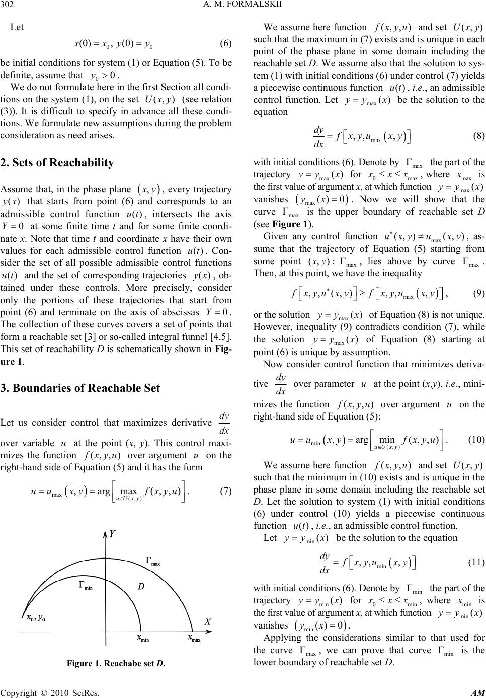

А. М. FORMALSKII 302
Let
00
(0), (0)
x
xy y (6)
be initial conditions for system (1) or Equation (5). To be
definite, assume that 00y.
We do not formulate here in the first Section all condi-
tions on the system (1), on the set (, )Uxy (see relation
(3)). It is difficult to specify in advance all these condi-
tions. We formulate new assumptions during the problem
consideration as need arises.
2. Sets of Reachability
Assume that, in the phase plane

,
x
y, every trajectory
()yx that starts from point (6) and corresponds to an
admissible control function ()ut, intersects the axis
0Y at some finite time t and for some finite coordi-
nate x. Note that time t and coordinate x have their own
values for each admissible control function ()ut . Con-
sider the set of all possible admissible control functions
()ut and the set of corresponding trajectories ()yx , ob-
tained under these controls. More precisely, consider
only the portions of these trajectories that start from
point (6) and terminate on the axis of abscissas 0Y

.
The collection of these curves covers a set of points that
form a reachable set [3] or so-called integral funnel [4,5].
This set of reachability D is schematically shown in Fig-
ure 1.
3. Boundaries of Reachable Set
Let us consider control that maximizes derivative dy
dx
over variable u at the point (x, y). This control maxi-
mizes the function (, , )
f
xyu over argument u on the
right-hand side of Equation (5) and it has the form

max (, )
,argmax(,,)
uU xy
uu xyfxyu





. (7)
Figure 1. Reachabe set D.
We assume here function (,, )
f
xyu and set (,)Uxy
such that the maximum in (7) exists and is unique in each
point of the phase plane in some domain including the
reachable set D. We assume also that the solution to sys-
tem (1) with initial conditions (6) under control (7) yields
a piecewise continuous function ()ut, i.e., an admissible
control function. Let max ()yy x

be the solution to the
equation

max
,, ,
dy
f
xyu xy
dx 



 (8)
with initial conditions (6). Denote by max
Γ the part of the
trajectory max ()yy x

for 0max
x
xx , where max
x
is
the first value of argument x, at which function max()yy x

vanishes


max ()0yx

. Now we will show that the
curve max Γ is the upper boundary of reachable set D
(see Figure 1).
Given any control function max (, )(, )uxy uxy
, as-
sume that the trajectory of Equation (5) starting from
some point max (, )Γxy

, lies above by curve max Γ.
Then, at this point, we have the inequality

max
,, (,),,,
f
xyu xyf xyuxy




 , (9)
or the solution max()yy x

of Equation (8) is not unique.
However, inequality (9) contradicts condition (7), while
the solution max ()yy x

of Equation (8) starting at
point (6) is unique by assumption.
Now consider control function that minimizes deriva-
tive dy
dx over parameter u at the point (x,y), i.e., mini-
mizes the function (,,)
f
xyu over argument u on the
right-hand side of Equation (5):

min (,)
,argmin(,,)
uU xy
uu xyfxyu





. (10)
We assume here function (,, )
f
xyu and set (, )Uxy
such that the minimum in (10) exists and is unique in the
phase plane in some domain including the reachable set
D. Let the solution to system (1) with initial conditions
(6) under control (10) yields a piecewise continuous
function ()ut , i.e., an admissible control function.
Let min ()yy x

be the solution to the equation

min
,, ,
dy
f
xyuxy
dx 



 (11)
with initial conditions (6). Denote by min
Γ the part of the
trajectory min ()yy x

for 0min
x
xx , where mi n
x
is
the first value of argument x, at which function min ()yy x

vanishes


min ()0yx

.
Applying the considerations similar to that used for
the curve max Γ, we can prove that curve min Γ is the
lower boundary of reachable set D.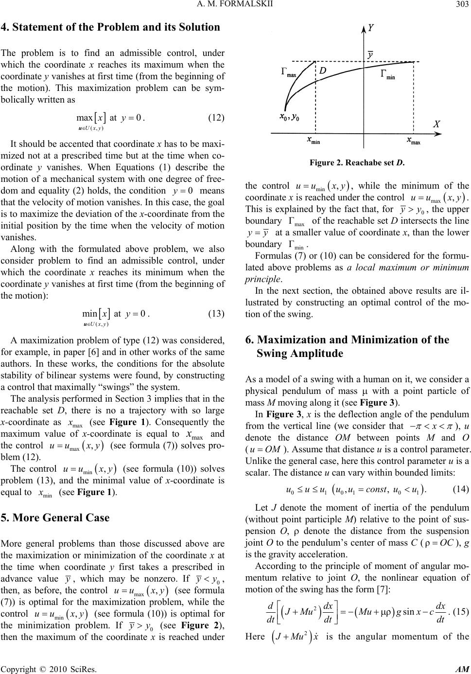

А. М. FORMALSKII 303
4. Statement of the Problem and its Solution
The problem is to find an admissible control, under
which the coordinate x reaches its maximum when the
coordinate y vanishes at first time (from the beginning of
the motion). This maximization problem can be sym-
bolically written as


(,)
max at 0
Uxy
xy


u
. (12)
It should be accented that coordinate x has to be maxi-
mized not at a prescribed time but at the time when co-
ordinate y vanishes. When Equations (1) describe the
motion of a mechanical system with one degree of free-
dom and equality (2) holds, the condition 0y means
that the velocity of motion vanishes. In this case, the goal
is to maximize the deviation of the x-coordinate from the
initial position by the time when the velocity of motion
vanishes.
Along with the formulated above problem, we also
consider problem to find an admissible control, under
which the coordinate x reaches its minimum when the
coordinate y vanishes at first time (from the beginning of
the motion):


(,)
min at 0
Uxy
xy


u
. (13)
A maximization problem of type (12) was considered,
for example, in paper [6] and in other works of the same
authors. In these works, the conditions for the absolute
stability of bilinear systems were found, by constructing
a control that maximally “swings” the system.
The analysis performed in Section 3 implies that in the
reachable set D, there is no a trajectory with so large
x-coordinate as max
x
(see Figure 1). Consequently the
maximum value of x-coordinate is equal to max
x
and
the control

max ,uu xy (see formula (7)) solves pro-
blem (12).
The control

min ,uu xy (see formula (10)) solves
problem (13), and the minimal value of x-coordinate is
equal to min
x
(see Figure 1).
5. More General Case
More general problems than those discussed above are
the maximization or minimization of the coordinate x at
the time when coordinate y first takes a prescribed in
advance value
y
, which may be nonzero. If 0 yy

,
then, as before, the control

max ,uu xy (see formula
(7)) is optimal for the maximization problem, while the
control

min ,uu xy (see formula (10)) is optimal for
the minimization problem. If 0 yy (see Figure 2),
then the maximum of the coordinate x is reached under
Figure 2. Reachabe set D.
the control


min ,uu xy, while the minimum of the
coordinate x is reached under the control


max ,uu xy.
This is explained by the fact that, for 0 yy, the upper
boundary max Γ of the reachable set D intersects the line
y
y

at a smaller value of coordinate x, than the lower
boundary min Γ.
Formulas (7) or (10) can be considered for the formu-
lated above problems as a local maximum or minimum
principle.
In the next section, the obtained above results are il-
lustrated by constructing an optimal control of the mo-
tion of the swing.
6. Maximization and Minimization of the
Swing Amplitude
As a model of a swing with a human on it, we consider a
physical pendulum of mass  with a point particle of
mass M moving along it (see Figure 3).
In Figure 3, x is the deflection angle of the pendulum
from the vertical line (we consider that
x

  ), u
denote the distance OM between points M and O
(uOM

). Assume that distance u is a control parameter.
Unlike the general case, here this control parameter u is a
scalar. The distance u can vary within bounded limits:


0101 01
,, .uuuuuconstuu (14)
Let J denote the moment of inertia of the pendulum
(without point participle M) relative to the point of sus-
pension O,  denote the distance from the suspension
joint O to the pendulum’s center of mass C (ρOC

), g
is the gravity acceleration.
According to the principle of moment of angular mo-
mentum relative to joint O, the nonlinear equation of
motion of the swing has the form [7]:


2ρsin
ddx dx
J
MuMugx c
dt dtdt



 . (15)
Here


2
J
Mu x is the angular momentum of the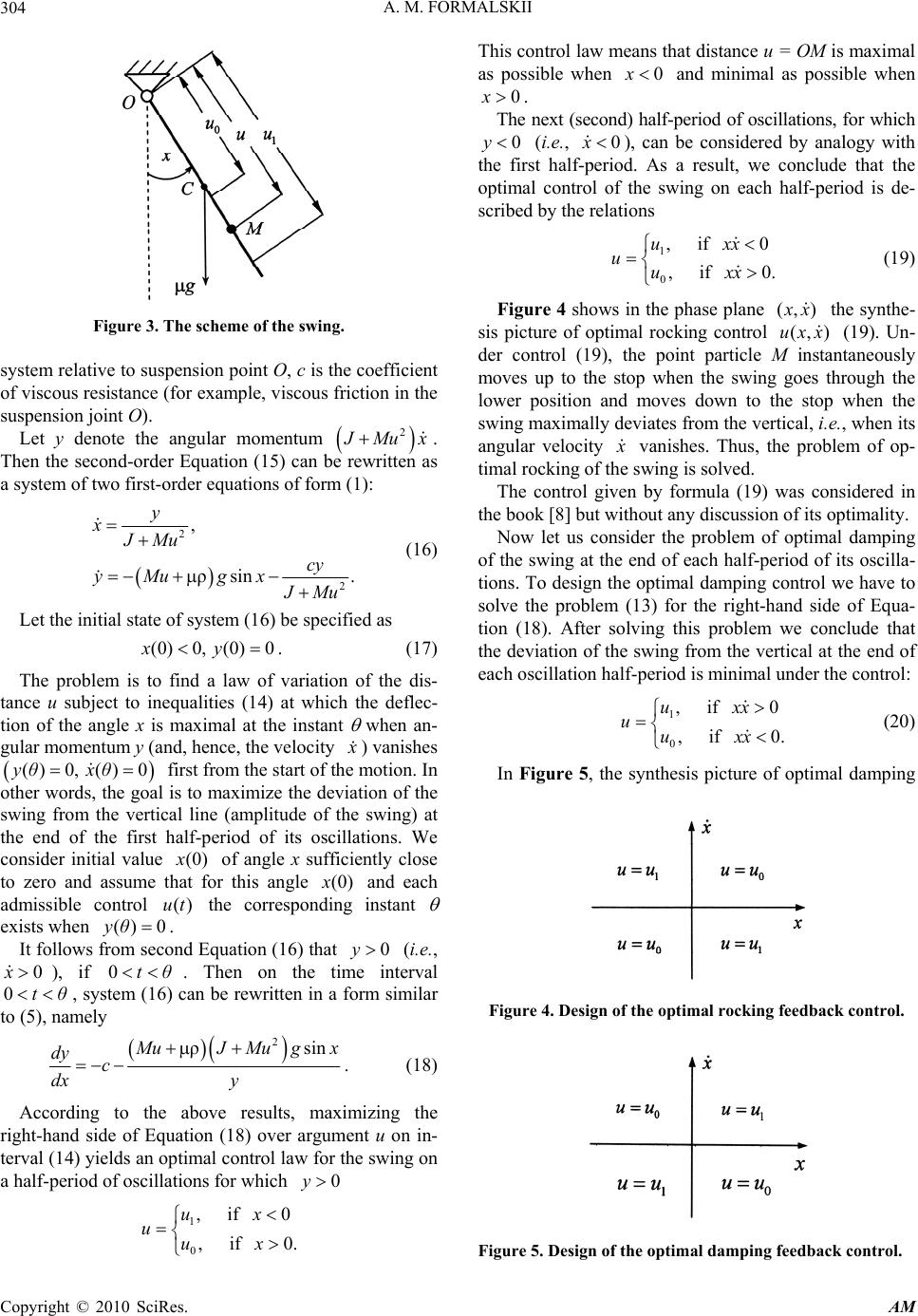

А. М. FORMALSKII 304
Figure 3. The scheme of the swing.
system relative to suspension point O, c is the coefficient
of viscous resistance (for example, viscous friction in the
suspension joint O).
Let y denote the angular momentum

2
J
Mu x.
Then the second-order Equation (15) can be rewritten as
a system of two first-order equations of form (1):

2
2
,
ρsin .
y
xJMu
cy
yMu gx
J
Mu

 


(16)
Let the initial state of system (16) be specified as
(0)0, (0)0xy. (17)
The problem is to find a law of variation of the dis-
tance u subject to inequalities (14) at which the deflec-
tion of the angle x is maximal at the instant
 when an-
gular momentum y (and, hence, the velocity
x
) vanishes

()0, ()0yθxθ
 first from the start of the motion. In
other words, the goal is to maximize the deviation of the
swing from the vertical line (amplitude of the swing) at
the end of the first half-period of its oscillations. We
consider initial value (0)
x
of angle x sufficiently close
to zero and assume that for this angle (0)
x
and each
admissible control ()ut the corresponding instant 
exists when ()0yθ.
It follows from second Equation (16) that 0y (i.e.,
0x
), if 0tθ . Then on the time interval
0tθ , system (16) can be rewritten in a form similar
to (5), namely


2
ρsin
M
uJMugx
dy c
dx y
 
 . (18)
According to the above results, maximizing the
right-hand side of Equation (18) over argument u on in-
terval (14) yields an optimal control law for the swing on
a half-period of oscillations for which 0y
1
0
, if 0
, if 0.
ux
uux




This control law means that distance u = OM is maximal
as possible when 0x

and minimal as possible when
0x.
The next (second) half-period of oscillations, for which
0y

(i.e., 0x

), can be considered by analogy with
the first half-period. As a result, we conclude that the
optimal control of the swing on each half-period is de-
scribed by the relations
1
0
, if 0
, if 0.
uxx
uuxx





 (19)
Figure 4 shows in the phase plane (,)
x
x
 the synthe-
sis picture of optimal rocking control (,)uxx
 (19). Un-
der control (19), the point particle M instantaneously
moves up to the stop when the swing goes through the
lower position and moves down to the stop when the
swing maximally deviates from the vertical, i.e., when its
angular velocity
x
 vanishes. Thus, the problem of op-
timal rocking of the swing is solved.
The control given by formula (19) was considered in
the book [8] but without any discussion of its optimality.
Now let us consider the problem of optimal damping
of the swing at the end of each half-period of its oscilla-
tions. To design the optimal damping control we have to
solve the problem (13) for the right-hand side of Equa-
tion (18). After solving this problem we conclude that
the deviation of the swing from the vertical at the end of
each oscillation half-period is minimal under the control:
1
0
, if 0
, if 0.
uxx
uuxx





 (20)
In Figure 5, the synthesis picture of optimal damping
Figure 4. Design of the optimal rocking feedback control.
Figure 5. Design of the optimal damping feedback control.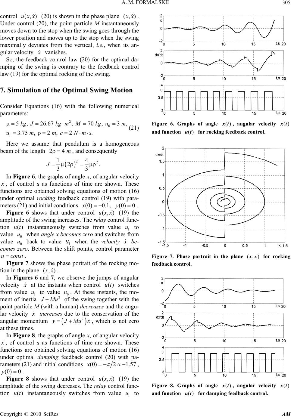

А. М. FORMALSKII 305
control (,)uxx
 (20) is shown in the phase plane (,)
x
x
.
Under control (20), the point particle M instantaneously
moves down to the stop when the swing goes through the
lower position and moves up to the stop when the swing
maximally deviates from the vertical, i.e., when its an-
gular velocity
x
 vanishes.
So, the feedback control law (20) for the optimal da-
mping of the swing is contrary to the feedback control
law (19) for the optimal rocking of the swing.
7. Simulation of the Optimal Swing Motion
Consider Equations (16) with the following numerical
parameters:
2
0
1
5 , 26.67 , 70 , 3 ,
3.75 , 2 , 2 .
kgJkg mMkgum
ummcNms
 
 (21)
Here we assume that pendulum is a homogeneous
beam of the length 4 m, and consequently

22
14
2
33
J



.
In Figure 6, the graphs of angle x, of angular velocity
x
, of control u as functions of time are shown. These
functions are obtained solving equations of motion (16)
under optimal rocking feedback control (19) with para-
meters (21) and initial conditions (0) 0.1x, (0) 0y

.
Figure 6 shows that under control (,)uxx
 (19) the
amplitude of the swing increases. The relay control func-
tion ()ut instantaneously switches from value 1
u to
value 0
u when angle x becomes zero and switches from
value 0
u back to value 1 u when the velocity
x
 be-
comes zero. Between the shift points, control parameter
u const.
Figure 7 shows the phase portrait of the rocking mo-
tion in the plane (,)
x
x
.
In Figures 6 and 7, we observe the jumps of angular
velocity
x
 at the instants when control ()ut switches
from value 1
u to value 0 u. At these instants, the mo-
ment of inertia 2
J
Mu of the swing together with the
point particle M (with a human) decreases and the angu-
lar velocity
x
 increases due to the conservation of the
angular momentum

2
yJMux , which is not zero
at these times.
In Figure 8, the graphs of angle x, of angular velocity
x
, of control u as functions of time are shown. These
functions are obtained solving equations of motion (16)
under optimal damping feedback control (20) with pa-
rameters (21) and initial conditions (0)2 1.57x

 ,
(0) 0y.
Figure 8 shows that under control (,)uxx
 (19) the
amplitude of the swing decreases. The relay control func-
tion ()ut instantaneously switches from value 1
u to
Figure 6. Graphs of angle ()xt , angular velocity ()

xt
and function ()ut for rocking feedback control.
Figure 7. Phase portrait in the plane (,)

xx for rocking
feedback control.
Figure 8. Graphs of angle ()xt , angular velocity ()  xt
and function ()ut for damping feedback control.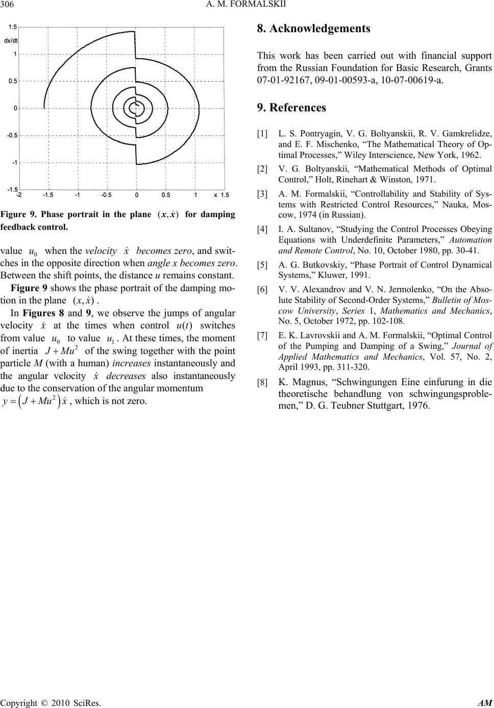

А. М. FORMALSKII 306
Figure 9. Phase portrait in the plane (,)

xx for damping
feedback control.
value 0
u when the velocity
x
 becomes zero, and swit-
ches in the opposite direction when angle x becomes zero.
Between the shift points, the distance u remains constant.
Figure 9 shows the phase portrait of the damping mo-
tion in the plane (,)
x
x
.
In Figures 8 and 9, we observe the jumps of angular
velocity
x
 at the times when control ()ut switches
from value 0 u to value 1 u. At these times, the moment
of inertia 2
J
Mu of the swing together with the point
particle M (with a human) increases instantaneously and
the angular velocity
x
 decreases also instantaneously
due to the conservation of the angular momentum

2
yJMux, which is not zero.
8. Acknowledgements
This work has been carried out with financial support
from the Russian Foundation for Basic Research, Grants
07-01-92167, 09-01-00593-a, 10-07-00619-а.
9. References
[1] L. S. Pontryagin, V. G. Boltyanskii, R. V. Gamkrelidze,
and E. F. Mischenko, “The Mathematical Theory of Op-
timal Processes,” Wiley Interscience, New York, 1962.
[2] V. G. Boltyanskii, “Mathematical Methods of Optimal
Control,” Holt, Rinehart & Winston, 1971.
[3] A. M. Formalskii, “Controllability and Stability of Sys-
tems with Restricted Control Resources,” Nauka, Mos-
cow, 1974 (in Russian).
[4] I. A. Sultanov, “Studying the Control Processes Obeying
Equations with Underdefinite Parameters,” Automation
and Remote Control, No. 10, October 1980, pp. 30-41.
[5] A. G. Butkovskiy, “Phase Portrait of Control Dynamical
Systems,” Kluwer, 1991.
[6] V. V. Alexandrov and V. N. Jermolenko, “On the Abso-
lute Stability of Second-Order Systems,” Bulletin of Mos-
cow University, Series 1, Mathematics and Mechanics,
No. 5, October 1972, pp. 102-108.
[7] E. K. Lavrovskii and A. M. Formalskii, “Optimal Control
of the Pumping and Damping of a Swing,” Journal of
Applied Mathematics and Mechanics, Vol. 57, No. 2,
April 1993, pp. 311-320.
[8] K. Magnus, “Schwingungen Eine einfurung in die
theoretische behandlung von schwingungsproble-
men,” D. G. Teubner Stuttgart, 1976.