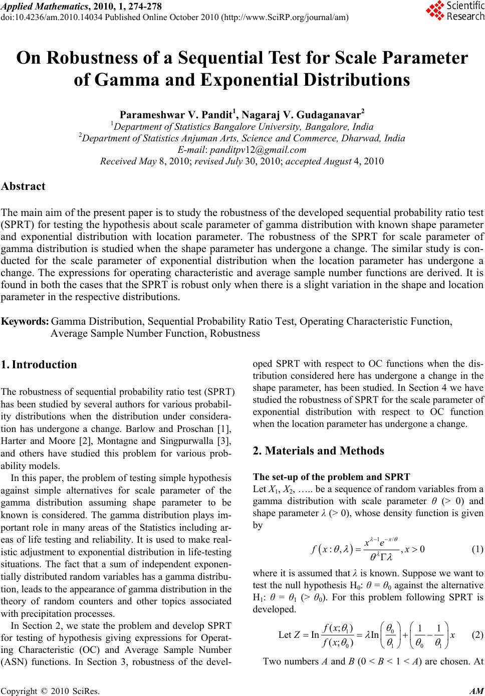Applied Mathematics, 2010, 1, 274-278
doi:10.4236/am.2010.14034 Published Online October 2010 (http://www.SciRP.org/journal/am)
On Robustness of a Sequential Test for Scale Parameter
of Gamma and Exponential Distribu tions
Parameshwar V. Pandit1, Nagaraj V. Gudaganava r2
1Department of Statistics Bangalore University, Bangalore, India
2Department of Statistics Anjuman Arts, Science and Commerce, Dharwad, India
Received May 8, 2010; revised July 30, 2010; accepted August 4, 2010
Abstract
The main aim of the present paper is to study the robustness of the developed sequential probability ratio test
(SPRT) for testing the hypothesis about scale parameter of gamma distribution with known shape parameter
and exponential distribution with location parameter. The robustness of the SPRT for scale parameter of
gamma distribution is studied when the shape parameter has undergone a change. The similar study is con-
ducted for the scale parameter of exponential distribution when the location parameter has undergone a
change. The expressions for operating characteristic and average sample number functions are derived. It is
found in both the cases that the SPRT is robust only when there is a slight variation in the shape and location
parameter in the respective distributions.
Keywords: Gamma Distribution, Sequential Probability Ratio Test, Operating Characteristic Function,
Average Sample Number Function, Robustness
1. Introduction
The robustness of sequential probability ratio test (SPRT)
has been studied by several authors for various probabil-
ity distributions when the distribution under considera-
tion has undergone a change. Barlow and Proschan [1],
Harter and Moore [2], Montagne and Singpurwalla [3],
and others have studied this problem for various prob-
ability models.
In this paper, the problem of testing simple hypothesis
against simple alternatives for scale parameter of the
gamma distribution assuming shape parameter to be
known is considered. The gamma distribution plays im-
portant role in many areas of the Statistics including ar-
eas of life testing and reliability. It is used to make real-
istic adjustment to exponential distribution in life-testing
situations. The fact that a sum of independent exponen-
tially distributed random variables has a gamma distribu-
tion, leads to the appearance of gamma distribution in the
theory of random counters and other topics associated
with precipitation processes.
In Section 2, we state the problem and develop SPRT
for testing of hypothesis giving expressions for Operat-
ing Characteristic (OC) and Average Sample Number
(ASN) functions. In Section 3, robustness of the devel-
oped SPRT with respect to OC functions when the dis-
tribution considered here has undergone a change in the
shape parameter, has been studied. In Section 4 we have
studied the robustness of SPRT for the scale parameter of
exponential distribution with respect to OC function
when the location parameter has undergone a change.
2. Materials and Methods
The set-up of the problem and SPRT
Let X1, X2, ….. be a sequence of random variables from a
gamma distribution with scale parameter θ (> 0) and
shape parameter λ (> 0), whose density function is given
by

1/
:,, 0
x
xe
fx x


 



 (1)
where it is assumed that λ is known. Suppose we want to
test the null hypothesis H0: θ = θ0 against the alternative
H1: θ = θ1 (> θ0). For this problem following SPRT is
developed.
0 1
0101
(; )11
Let InIn
(; )
fx
Z
x
fx
 

 

 


(2)
Two numbers A and B (0 < B < 1 < A) are chosen. At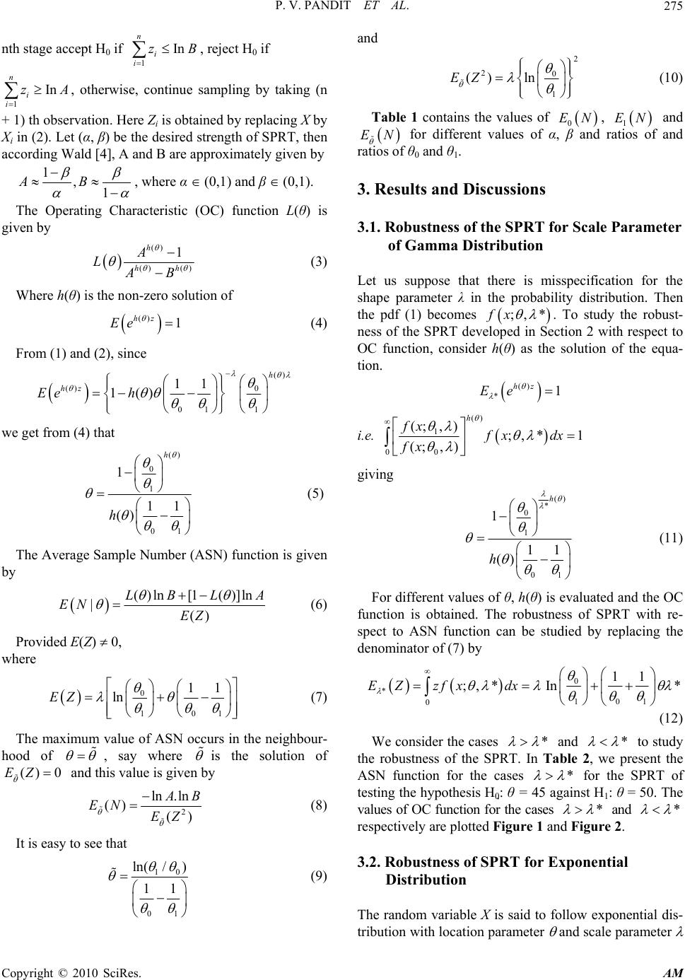

P. V. PANDIT ET AL. 275
nth stage accept H0 if
1
In
n
i
i
zB


, reject H0 if
1
In
n
i
i
zA


, otherwise, continue sampling by taking (n
+ 1) th observation. Here Zi is obtained by replacing X by
Xi in (2). Let (α, β) be the desired strength of SPRT, then
according Wald [4], A and B are approximately given by
1,1
AB






, where α  (0,1) and β  (0,1).
The Operating Characteristic (OC) function L(θ) is
given by

()
() ()
1
h
hh
A
LAB





 (3)
Where h(θ) is the non-zero solution of

() 1 hz
Ee

 (4)
From (1) and (2), since

()
() 0
01 1
11
1()
h
hz
Ee h





  


 

 
  

 

we get from (4) that
()
0
1
01
1
11
()
h
h














(5)
The Average Sample Number (ASN) function is given
by

()ln[1 ()]ln
|()
LBL A
EN EZ



 (6)
Provided E(Z)  0,
where

0
101
11
lnEZ




 

  

 

(7)
The maximum value of ASN occurs in the neighbour-
hood of

 , say where

is the solution of
() 0EZ


 and this value is given by
2
ln .ln
() ()
A
B
EN EZ






(8)
It is easy to see that
10
01
ln( /)
11









 (9)
and
2
20
1
() lnEZ











 (10)
Table 1 contains the values of


0
EN ,


1
EN and


EN

 for different values of α, β and ratios of and
ratios of θ0 and θ1.
3. Results and Discussions
3.1. Robustness of the SPRT for Scale Parameter
of Gamma Distribution
Let us suppose that there is misspecification for the
shape parameter λ in the probability distribution. Then
the pdf (1) becomes


;, *fx

 . To study the robust-
ness of the SPRT developed in Section 2 with respect to
OC function, consider h(θ) as the solution of the equa-
tion.


()
*1
hz
Ee



i.e.

()
1
0 0
(;, );, *1
(;, )
h
fx fx dx
fx

 

 



giving
()
*
0
1
01
1
11
()
h
h















(11)
For different values of θ, h(θ) is evaluated and the OC
function is obtained. The robustness of SPRT with re-
spect to ASN function can be studied by replacing the
denominator of (7) by
 
0
*
101
0
11
;,* In*EZ zfxdx



 




 



(12)
We consider the cases *

  and *

  to study
the robustness of the SPRT. In Table 2, we present the
ASN function for the cases *

  for the SPRT of
testing the hypothesis H0: θ = 45 against H1: θ = 50. The
values of OC function for the cases *

  and *



respectively are plotted Figure 1 and Figure 2.
3.2. Robustness of SPRT for Exponential
Distribution
The random variable X is said to follow exponential dis-
tribution with location parameter  and scale parameter 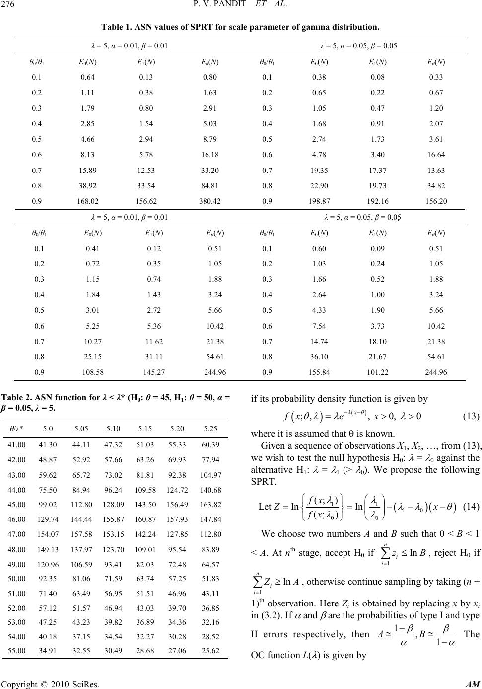

P. V. PANDIT ET AL. 276
Table 1. ASN values of SPRT for scale parameter of gamma distribution.
λ = 5, α = 0.01, β = 0.01 λ = 5, α = 0.05, β = 0.05
θ0/θ1 E0(N) E1(N) Eθ(N) θ0/θ1 E0(N) E1(N) Eθ(N)
0.1 0.64 0.13 0.80 0.1 0.38 0.08 0.33
0.2 1.11 0.38 1.63 0.2 0.65 0.22 0.67
0.3 1.79 0.80 2.91 0.3 1.05 0.47 1.20
0.4 2.85 1.54 5.03 0.4 1.68 0.91 2.07
0.5 4.66 2.94 8.79 0.5 2.74 1.73 3.61
0.6 8.13 5.78 16.18 0.6 4.78 3.40 16.64
0.7 15.89 12.53 33.20 0.7 19.35 17.37 13.63
0.8 38.92 33.54 84.81 0.8 22.90 19.73 34.82
0.9 168.02 156.62 380.42 0.9 198.87 192.16 156.20
λ = 5, α = 0.01, β = 0.01 λ = 5, α = 0.05, β = 0.05
θ0/θ1 E0(N) E1(N) Eθ(N) θ0/θ1 E0(N) E1(N) Eθ(N)
0.1 0.41 0.12 0.51 0.1 0.60 0.09 0.51
0.2 0.72 0.35 1.05 0.2 1.03 0.24 1.05
0.3 1.15 0.74 1.88 0.3 1.66 0.52 1.88
0.4 1.84 1.43 3.24 0.4 2.64 1.00 3.24
0.5 3.01 2.72 5.66 0.5 4.33 1.90 5.66
0.6 5.25 5.36 10.42 0.6 7.54 3.73 10.42
0.7 10.27 11.62 21.38 0.7 14.74 18.10 21.38
0.8 25.15 31.11 54.61 0.8 36.10 21.67 54.61
0.9 108.58 145.27 244.96 0.9 155.84 101.22 244.96
Table 2. ASN function for λ < λ* (H0: θ = 45, H1: θ = 50, α =
β = 0.05, λ = 5.
θ/λ* 5.0 5.05 5.10 5.15 5.20 5.25
41.00 41.30 44.11 47.3251.03 55.33 60.39
42.00 48.87 52.92 57.6663.26 69.93 77.94
43.00 59.62 65.72 73.0281.81 92.38 104.97
44.00 75.50 84.94 96.24109.58 124.72 140.68
45.00 99.02 112.80 128.09143.50 156.49 163.82
46.00 129.74 144.44 155.87160.87 157.93 147.84
47.00 154.07 157.58 153.15142.24 127.85 112.80
48.00 149.13 137.97 123.70109.01 95.54 83.89
49.00 120.96 106.59 93.4182.03 72.48 64.57
50.00 92.35 81.06 71.5963.74 57.25 51.83
51.00 71.40 63.49 56.9551.51 46.96 43.11
52.00 57.12 51.57 46.9443.03 39.70 36.85
53.00 47.25 43.23 39.8236.89 34.36 32.16
54.00 40.18 37.15 34.5432.27 30.28 28.52
55.00 34.91 32.55 30.4928.68 27.06 25.62
if its probability density function is given by


;,, 0, 0
x
fxe x

 


 (13)
where it is assumed that  is known.
Given a sequence of observations X1, X2, …, from (13),
we wish to test the null hypothesis H0:
 = 
0 against the
alternative H1:
 = 
1 (>

0). We propose the following
SPRT.
 
11
10
00
(; )
Let InIn
(; )
fx
Zx
fx







 
 (14)
We choose two numbers A and B such that 0 < B < 1
< A. At nth stage, accept H0 if
1
In
n
i
i
zB


, reject H0 if
1
ln
n
i
i
Z
A


, otherwise continue sampling by taking (n +
1)th observation. Here Zi is obtained by replacing x by xi
in (3.2). If
 and  are the probabilities of type I and type
II errors respectively, then 1,1
AB






The
OC function L(  ) is given by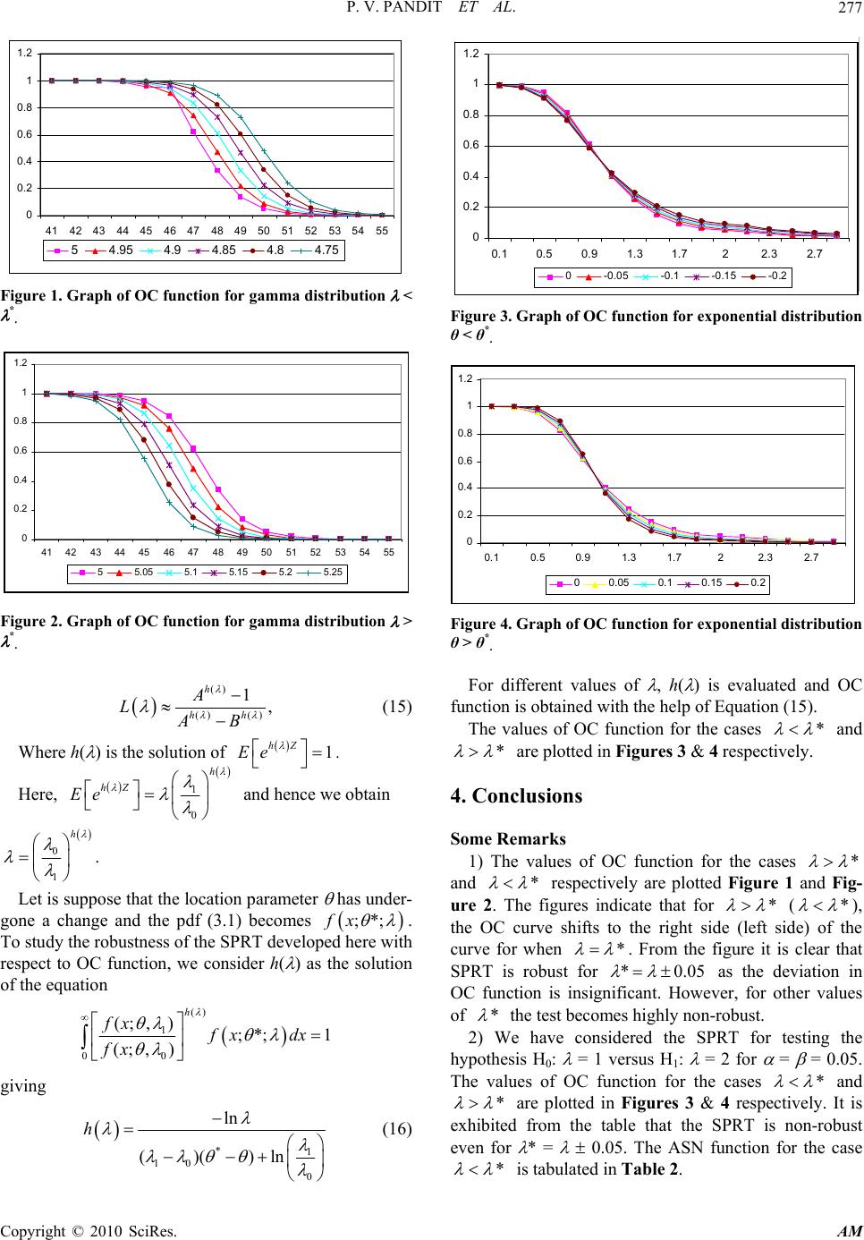

P. V. PANDIT ET AL. 277
0
0.2
0.4
0.6
0.8
1
1.2
41 42 43 4445 4647 484950 51525354 55
54.95 4.9 4.85 4.8 4.75
Figure 1. Graph of OC function for gamma distribution  <

*.
0
0.2
0.4
0.6
0.8
1
1.2
41 4243 44 4546 4748 49 5051 5253 54 55
55.05 5.1 5.15 5.2 5.25
Figure 2. Graph of OC function for gamma distribution  >

*.

()
() ()
1,
h
hh
A
LAB




 (15)
Where h(
 ) is the solution of

1
hZ
Ee




.
Here,



1
0
h
hZ
Ee








 and hence we obtain

0
1
h





.
Let is suppose that the location parameter  has under-
gone a change and the pdf (3.1) becomes

;*;fx

 .
To study the robustness of the SPRT developed here with
respect to OC function, we consider h(
 ) as the solution
of the equation

()
1
0 0
(; ,);*; 1
(; ,)
h
fx fx dx
fx

 

 



giving

*1
10
0
ln
()()ln
h










(16)
0
0.2
0.4
0.6
0.8
1
1.2
0.10.5 0.9 1.31.722.3 2.7
0-0.05 -0.1 -0.15 -0 .2
Figure 3. Graph of OC function for exponential distr i bution
θ < θ*.
0
0. 2
0. 4
0. 6
0. 8
1
1. 2
0.1 0.50.9 1.3 1.722.3 2.7
00.05 0.1 0.15 0.2
Figure 4. Graph of OC function for exponential distr i bution
θ > θ*.
For different values of  , h(  ) is evaluated and OC
function is obtained with the help of Equation (15).
The values of OC function for the cases *



and
*

  are plotted in Figures 3 & 4 respectively.
4. Conclusions
Some Remarks
1) The values of OC function for the cases *

 
and *



respectively are plotted Figure 1 and Fig-
ure 2. The figures indicate that for *

  (*



),
the OC curve shifts to the right side (left side) of the
curve for when *



. From the figure it is clear that
SPRT is robust for *0.05



 as the deviation in
OC function is insignificant. However, for other values
of *

the test becomes highly non-robust.
2) We have considered the SPRT for testing the
hypothesis H0:  = 1 versus H1:  = 2 for  =  = 0.05.
The values of OC function for the cases *



and
*

  are plotted in Figures 3 & 4 respectively. It is
exhibited from the table that the SPRT is non-robust
even for  * =   0.05. The ASN function for the case
*



is tabulated in Table 2.

P. V. PANDIT ET AL. 278
5. References
[1] R. E. Barlow and E. Proschan, “Exponential Life Test
Procedures When the Distribution under Test has Mono-
tone Failure Rate,” Journal of American Statistic Asso-
ciation, Vol. 62, No. 318, 1967, pp. 548-560.
[2] L. Harter and A. H. Moore, “An Evaluation of Exponen-
tial and Weibull Test Plans,” IEEE Transactions on Re-
liability, Vol. 25, No. 2, 1976, pp. 100-104.
[3] E. R. Montagne and N. D. Singpurwalla, “Robustness of
Sequential Exponential Life-Testing Procedures,” Jour-
nal of American Statistic Association, Vol. 80, No. 391,
1985, pp. 715-719.
[4] A. Wald, “Sequential Analysis,” John Wiley, New York,
1947.