Open Journal of Fluid Dynamics
Vol.2 No.4A(2012), Article ID:26371,7 pages DOI:10.4236/ojfd.2012.24A047
Performances of Volume-PTV and Tomo-PIV
1Division of Mechanical and Energy Systems Engineering, Korea Maritime University, Busan, South Korea
2LG Electronics, Home Appliance, Changwon, South Korea
Email: doh@hhu.ac.kr
Received October 3, 2012; revised November 14, 2012; accepted November 24, 2012
Keywords: Volume-Particle-Tracking Velocimetry; Tomographic-Particle Image Velocimetry; Ring Vortex; Recovery Ratio
ABSTRACT
We constructed a volume particle-tracking velocimetry (Volume-PTV) algorithm for comparisons with the tomographic particle image velocimetry (Tomo-PIV) algorithm, in which the multiplicative algebraic reconstruction technique (MART) was adopted. Performance tests on both algorithms were conducted by using artificial images generated through numerical data sets. Standard data on an impinging jet were used to test the Volume-PTV algorithm, whereas ring vortex data were used to test the Tomo-PIV algorithm. The influence of the number of particles (particle density in volume) on the key factors of Volume-PTV, such as particle movements and particle neighborhoods, were investigated. Furthermore, the effects of particle density and sizes onto the recovery ratio of the vectors were evaluated.
1. Introduction
A large number of studies have attempted to obtain quantitative 3D information from flow fields. Several studies on stereo particle image velocimetry (PIV) have shown the capability of the PIV technique in visualizing complex flows quantitatively [1,2]. Hinsch [3] and Chan et al. [4] verified the possibility of the quantification of complex flows by holographic PIV (HPIV). The reconstructed intensity field was scanned by a charge-coupled device (CCD) sensor. However, the recording medium was a holographic film that requires wet processing. This process is time consuming and inaccurate because of the misalignment and distortion produced when re-positioning the hologram for object reconstruction. Hologram recording on a photographic plate can also be captured directly by a CCD sensor such as a digital HPIV (DHPIV) [5]. In this case, the light intensity distribution in the measurement volume is built numerically by solving the Fresnel diffraction formula for holographic near-field diffraction [6]. However, CCD sensors have very limited resolutions compared with photographic plates, returning about 2 to 3 orders less of particle images and velocity vectors. The large pixel pitch requires the recording to be obtained at a relatively small angle (a few degrees between the reference beam and scattered light) to resolve the interference pattern, thereby strongly limiting the numerical aperture and depth resolution [3]. Kim and Lee [7] constructed an in-line DHPIV by introducing a highdefinition camera (1 K × 1 K). The authors evaluated the maximum possible particle density of in-line DHPIVs. The results show that the recovery ratio (RR) of the whole particles in the measurement volume is approximately 65% when the particle density is 25 mm3. This result indicates that the identifiable number of whole particles is approximately 8500 among the 13,000 particles in the measurement volume.
Scarano et al. [8] developed a tomographic-PIV (TomoPIV). The Tomo-PIV was used for measuring a cylinder wake with a measurement volume of 80 mm × 80 mm × 15 mm. This algorithm was developed to increase the measurable number of vectors. Doh et al. [9,10] developed a genetic algorithm based on 3D particle-tracking velocimetry (3D-PTV) for measuring a cylinder wake with a volume of 50 mm × 50 mm × 50 mm. The authors obtained over 10,000 instantaneous vectors with a 1 K × 1 K camera. Lai et al. [11] developed a defocused 3DPTV with a measurable volume of 100 mm × 100 mm × 100 mm. Based on the number of vectors, the density of vectors per unit volume (1 mm3) obtained by the defocused 3D-PTV is more sparse than the one obtained by the DHPIV and Volume-PIV. The measured volume size of 3D-PTVs and Volume PIVs can be adjusted to that of HPIV by employing an optimized optical arrangement; thus, the identifiable particle numbers in the same particle density can be regarded as identical. The measureable thickness of the Volume-PIVs is restricted to a certain length because of the loss of image information, which is caused by an increase in the uncertainty of particle volume patterns with increasing camera-viewing depth. The drawbacks of 3D-PTVs are the numerous spurious vectors that exist among the calculated vectors and the long calculation time. No report has been made regarding the most appropriate method for various flow measurements. This study compared the efficiency of the Volume-PTV and Tomo-PIV algorithms in measuring complex flow fields.
2. Volume-PTV and Tomo-PIV
2.1. 3D Measurement Principle
A 3D measurement can be attained by matching the captured images of two or more cameras. To match the images, precise identification of the coordinate relations between the photographical coordinates of the cameras and the physical coordinates is required. Therefore, camera calibrations were conducted to determine these relations. The 10-parameter method [9] was used to obtain six exterior parameters (dis, α, β, γ, mx, my) and four interior parameters (cx, cy, k1, k2). The variables (α, β, γ) represent the tilting angles of the photographic coordinates for the absolute axes. The collinear equation for every point between the two coordinates is expressed in the following equation.
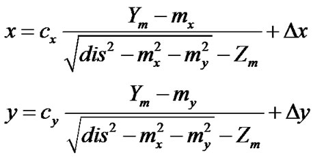 (1)
(1)
Variables cx and cy are the focal distances for the x and y components of the coordinate, respectively. Δx and Δy are the lens distortions and can be calculated by the following equation.
 (2)
(2)
Equation (2) can be converted into the following Equation (3).
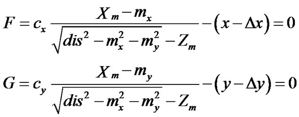 (3)
(3)
The study of Doh et al. [9,10] can be used as a reference for additional detailed calculation processes in obtaining camera parameters.
2.2. Volume-PTV
Figure 1 shows the developmental procedure for the Volume-PTV. After camera calibrations, 2D temporal vector trajectories for the whole particle pairs appeared on one camera image. The principle of finding the 2D vector trajectories is based on the 2D-PTV [12]. After obtaining the 2D vector candidates for each camera image, candidate trees were constructed by using the following hybrid fitness function (Figure 2).
 (4)
(4)
where x is the scale sensitivity factor (x = δ/PF; Figure 2). δ is calculated using this equation.
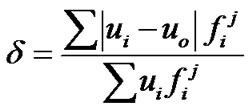 (5)
(5)
where, 
 ,
,
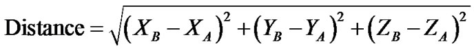
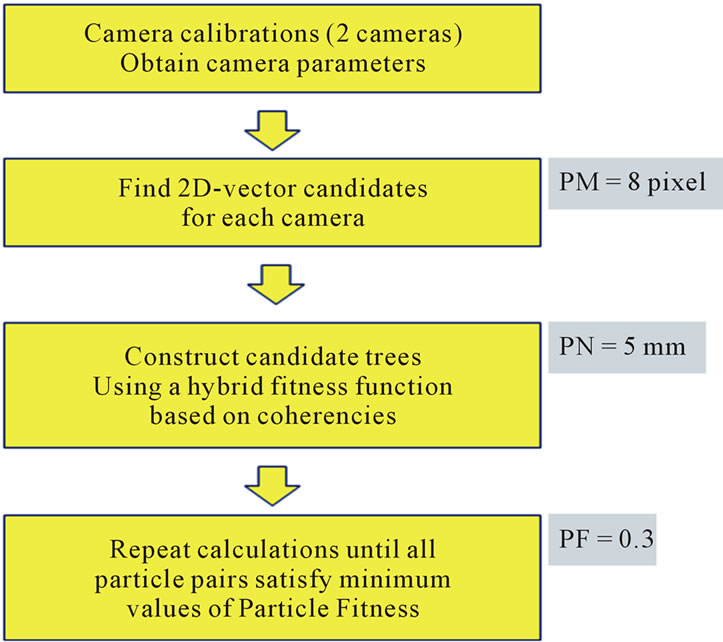
Figure 1. Overall procedure for Volume-PTV.
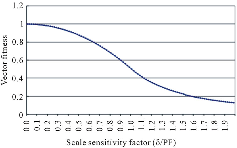
Figure 2. Fitness function against spatial distance.
where  represents the velocity vectors comprising all candidate vectors, and
  represents the mean vector of nearby vectors in a certain area. The formula
  was calculated repeatedly until the maximum value of each particle was obtained.
Particle fitness (PF) indicates the data range, in which outliers are eliminated (Figure 2). Data from this PF value were not sorted into the correct candidate data group. Figure 3 shows the concept of the PF value.  is the mean value of the velocity vectors in a certain searching region (Figure 4). A large PF value corresponds to large data variations in the correct data group. In other words, a larger PF value is recommended if the flow field is very complex and has a wide dynamic range.
Particle movement (PM) and particle neighborhood (PN) values are represented in [pixel] and [mm], respecttively. PM was used for finding the 2D particle trajectories of the same camera.
2D velocity vectors were installed within the PM [pixel] range, and all trajectories were stored in a candidate group. PM value was also used for other camera images. PN value was used for finding the same pairs in 3D space. As shown in Figure 4, particles in a sphere volume are regarded as one of the candidates and are subsequently sorted into the candidate group. The above-mentioned procedures indicate that two sets of 2D trajectories (i.e., 2D vectors) for the candidate data set were obtained from two camera images. The last data sets satisfied the PM and PN values.
2.3. Tomo-PIV
The principle of Tomo-PIV is based on the study of Elsinga et al. [13], except for the camera calibration process. Figure 5 shows the schematics of the Tomo-PIV. Tracer particles immersed in the flow were illuminated by a pulsed light source within a 3D region of space. The scattered light pattern was recorded simultaneously from several viewing directions using multiple cameras by applying the Scheimpflug condition on the image, lens, and mid-object plane. The particles within the entire volume have to be focused by setting a proper focal

Figure 3. Definition of the PF value.

Figure 4. Relations between particle searching region, particle neighborhood (PN), and particle movement (PM).
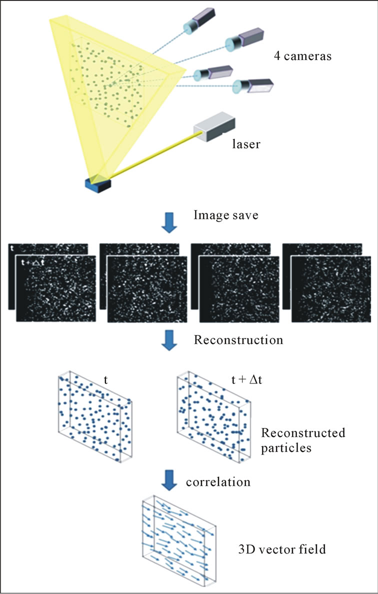
Figure 5. Principle of Tomo-PIV.
number. The 3D particle distribution (the object) was reconstructed as 3D light intensity distribution through the projections from the CCD arrays.
After reconstructing the whole images in virtual space, a voxel image was obtained. Thereafter, the cross-correlation of the particle intensity of the particles was calculated and the 3D vectors obtained on grids.
Figure 6 shows the relations between the projections
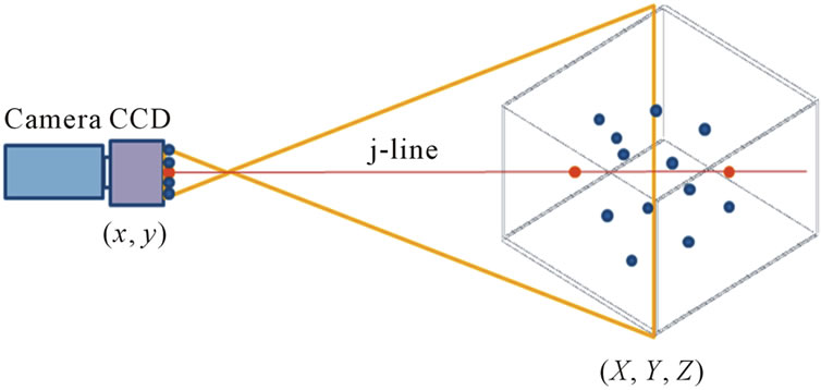
Figure 6. Relationship between voxel intensity and image intensity.
of the light intensity distribution, voxel intensity E(X, Y, Z), and image pixel (xi and yi). The light intensity distribution returns the pixel image intensity I(xi and yi; obtained from the recorded images), which can be written as the following linear equation.
 (6)
(6)
where Ni indicates the voxels intercepted or in the neighborhood of the line of sight corresponding to the ith pixel (xi, yi). The weighting coefficient wi,j describes the contribution of the jth voxel from intensity 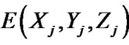 to pixel intensity I(xi, yi.). wi,j was calculated as the intersecting volume between the voxel and the line of sight (cross sectional area of the pixel) normalized with the voxel volume.
The coefficients depend on the relative size of a voxel to a pixel and the distance between the voxel center and the line of sight (Figure 6). Note that  for all wi,j entries in the 2D array. The weighting coefficients can also be used to account for different camera sensitivities, forward or backward scatter differences, or other optical dissimilarities between the cameras. wi,j was calculated based on the following Equation (7) and defined in Figure 7" target="_self"> Figure 7.
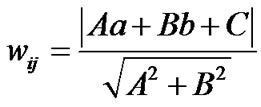 (7)
(7)
Equation (7) presents the distance between the voxel and the Epipolar line, which are constructed in 3D space. If the voxel location is far from the Epipolar line, the value of wi,j is set as a small value. Tomographic reconstruction was based on multiplicative algebraic reconstruction technique (MART) [14].
Equation (8) was used for calculating MART. The initial value for is set at one.
 (8)
(8)
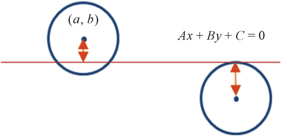
Figure 7. Epipolar line and distance.
Here, μ is a scalar relaxation parameter; the results of this parameter should be less than one. The magnitude of the update was determined by the ratio of the measured pixel intensity I with the projection of the current object . The exponent ensures the update of elements in E(X, Y, Z) that only affect the ith pixel. The MART scheme requires that E and I are definite positive.
2.4. Performance Comparison
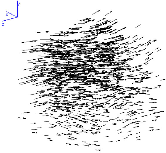
Performance tests were performed for Volume-PTV and Tomo-PIV. The large eddy simulation (LES) vector data sets by Okamoto et al. [14] were employed for the Volume-PTV, whereas a theoretically generated ring vortex data set was used for Tomo-PIV. Figure 8(a) shows the used 3D data of the impinging jet. Figure 8(b) shows the used 3D data of the generated ring vortex with the generation conditions using Equation (8).
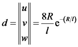 (9)
(9)
Here, d indicates the displacement of the vectors in the ring vortex. R and l indicate the radius and the thickness of the ring vortex as shown in Figure 8(b).
Figure 9 shows one of the generated artificial images of the ring vortex. Instantaneous vectors were randomly sampled by interpolating the LES data into space. The virtual image was generated using the selected vector data with a resolution of 1 K × 1 K pixels. Considering the centroids of the virtual images of particles, 3D vectors were calculated by the constructed algorithm. The generation procedures of virtual images in this study are similar to those by Okamoto et al. [14]. For the case of ring vortex tests, the image resolution was set to 700 × 700 pixel for both Volume-PTV and Tomo-PIV. Particle density was set at 0.05 particle per pixel (ppp). The measurement volume was set to 35 × 35 × 7 mm3.
Figure 10 shows the relationship between the PM [pixel] values and RR [%] of the velocity vectors. RR is defined as the amount of recovered (identified) vectors among the number of particles used for 3D vector calculation. The RR is significantly dependent on the number of particles and on the PM values when the distance error
 (a)
(a)  (b)
(b)
Figure 8. Data sets used for the performance tests of Volume-PTV and Tomo-PIV. (a) Impinging jet provided by Visualization Society of Japan (http://www.vsj.or.jp/piv) for Standard Image Test Project; (b) Ring vortex generated numerically. (a) Impinging jet; (b) Ring vortex.
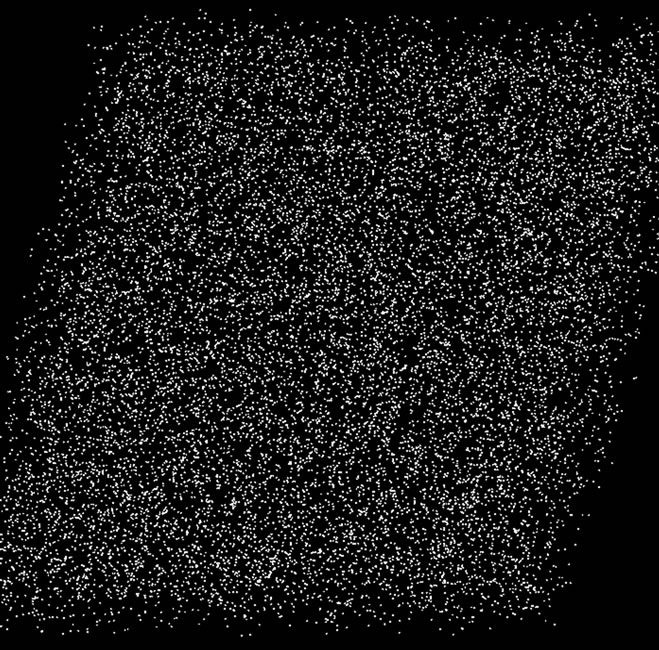
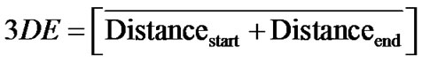
Figure 9. Generated artificial image for ring vortex.
(DE) value in the Equation (5) is small (0.2 mm). By contrast, the RR values are independent of the PM values when the DE value is large (2.0 mm).
Figure 11 presents the relationship between the PN [mm] values and the RR [%] at DE = 2.0 mm and PM = 7 pixels. The RR values are not dependent on the PN values but are strongly dependent on the number of particles.
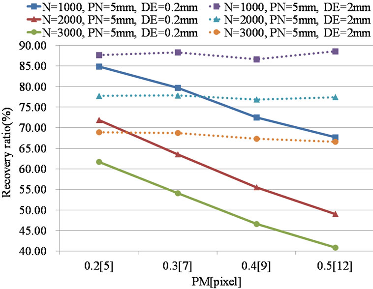
Figure 10. RR vs PM value (Volume-PTV) (N = 1000, 2000, 3000; PM = 5, 7, 9, 12 pixels; PN = 5 mm; DE = 0.2 mm, 2.0 mm).

Figure 11. RR vs PN value (Volume-PTV). (N = 1000, 2000, 3000; PM = 7 pixels; DE = 2.0 mm).
Figure 12 shows the relationship between the DE [mm] values and the RR [%] at PM = 5 pixels and PN = 5 mm. The RR values are significantly dependent on the number of particles and are saturated over DE = 0.4 mm. This result implies that the RR is only dependent on the density of a particle if the DE values are higher than 0.4 mm.
Figure 13 presents the relationship between the number of particles and the RR [%] at PN = 5 mm with changes in the PM values (5, 7, 9, and 12 pixels). At DE = 2.0 mm, the RR values are approximately 10% to 30% larger for all particle densities. The RR values increased with decreasing PM values at the same particle number. The RR of the velocity vectors obtained in the actual experiment is slightly smaller than the results obtained in the performance test.
Figure 14 shows the reconstructed vector fields obtained
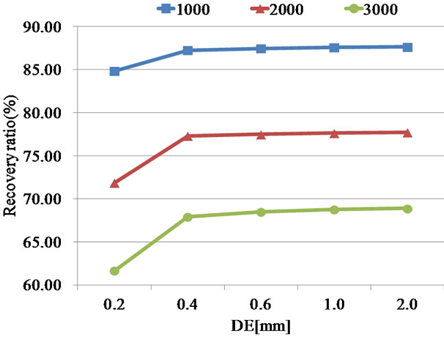
Figure 12. RR vs DE value (Volume-PTV) (N = 1000, 2000, 3000; PM = 5 pixels, PN = 5 mm).

Figure 13. RR vs particle number with PM value (N = 1000, 2000, 3000; PM = 5, 7, 9, 12 pixels; PN = 5 mm; DE = 0.2 mm, 2.0 mm).
by the constructed Tomo-PIV. The reconstructed vector field is almost the same as that of the theoretical one (Figure 8). Figure 15 shows that the voxel error changes with changing particle density at several particle sizes. The voxel errors are independent of the particle density [voxel/frame] when the particle size is 1 pixel. However, the voxel errors increase with increasing particle density when particle sizes are over 1.5 pixels. At a particle size of 3 pixels, the voxel errors significantly increase with increasing particle density. Figure 16 shows that the voxel error changes with changing particle size at several particle densities. The voxel errors slightly increase with increasing particle size when the particle size is over 1.5 pixels. However, the error increments increase with increasing particle density. The voxel errors increase very slightly at a particle density of 0.02 voxel/frame.
3. Conclusions
We constructed a Volume-PTV and tested its performance for the impinging jet flow and the ring vortex flow, whereas a Tomo-PIV was also constructed and its performance was evaluated for the same flows. The summary of the results is presented as follows.
1) Measurement results obtained by the Tomo-PIV are

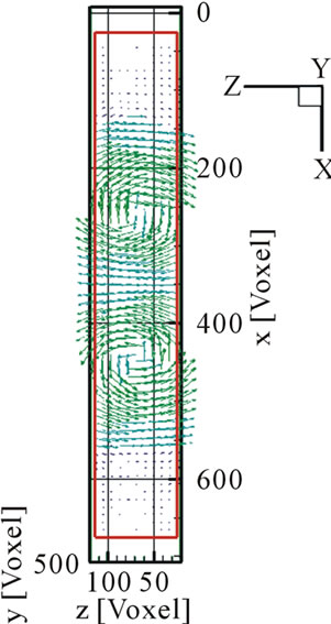
Figure 14. Reconstructed ring vortex.

Figure 15. Error changes in particle density (Tomo-PIV).

Figure 16. Error changes in particle size (Tomo-PIV).
qualitatively better than those of the Volume-PTV under the same camera locations. However, the results obtained by the Volume-PTV can be significantly improved by setting the cameras at a large viewing angle and by increasing the number of cameras;
2) For Volume-PTV, the RR of vectors is strongly dependent on particle density. The optimal parameters are PM = 8 pixels, PN = 5 mm, and PF = 0.3. With these parameters, more than 10,000 vectors can be obtained corresponding to 65% to 70% of the vector RR. VolumePTV is significantly affected by the location of the cameras;
3) For Tomo-PIV, the voxel errors increase with increasing particle density. The voxel errors are smallest when the particle size is between 1.0 pixel to 2.0 pixels. A particle size smaller than 3 pixels is preferable.
4. Acknowledgements
This work was supported by the National Research Foundation (NRF) of Korea grant funded by the MEST of Korea (No. 2008-0060153).
REFERENCES
- M. P. Arroyo and C. A. Greated, “Stereoscopic Particle Image Velocimetry,” Measurement Science and Technology, Vol. 2, No. 12, 1991, pp. 1181-1186. doi:10.1088/0957-0233/2/12/012
- C. J. Kähler and J. Kompenhans, “Fundamentals of Multiple Plane Stereo Particle Image Velocimetry,” Experiment in Fluids, Vol. 29, No. 1, 2000, pp. S70-S77. doi:10.1007/s003480070009
- K. D. Hinsch and S. F. Herrmann “Holographic Particle Image Velocimetry,” Measurement Science and Technology, Vol. 15, No. 4, 2002, pp. R61-R72. doi:10.1088/0957-0233/15/4/E01
- V. S. S. Chan, W. D. Koek, D. H. Barnhart, N. Bhattacharya, J. J. M. Braat and J. Westerweel, “Application of Holography to Fluid Flow Measurements using Bacteriorhodopsin,” Measurement Science and Technology, Vol. 15, No. 4, 2004, pp. 647-655. doi:10.1088/0957-0233/15/4/006
- S. Coëtmellec, C. Buraga-Lefebvre, D. Lebrun and C. Özkul, “Application of In-Line Digital Holography to Multiple Plane Velocimetry,” Measurement Science and Technology, Vol. 12, No. 9, 2001, pp. 1392-1397. doi:10.1088/0957-0233/12/9/303
- G. Pan and H. Meng, “Digital Holography of Particle Fields: Reconstruction by Use of Complex Amplitude,” Applied Optics, Vol. 42, No. 5, 2002, pp. 827-833.
- S. Kim and S. J. Lee, “Effect of Particle Number Density in In-line Digital Holographic Particle Velocimetry,” Experiment in Fluids, Vol. 44, No. 4, 2008, pp. 623-631. doi:10.1007/s00348-007-0422-z
- F. Scarano, G. E. Elsinga, E. Bocci and B. W. van Oudheusden, “Investigation of 3-D Coherent Structures in the Turbulent Cylinder Wake using Tomo-PIV,” CD-ROM Proceedings of 13th International Symposium on Applications of Laser Techniques to Fluid Mechanics, Lisbon, 26-29 June 2006, pp. 1-11.
- D. H. Doh, T. G. Hwang and T. Saga, “3D-PTV Measurements of the Wake of a Sphere,” Measurement Science and Technology, Vol. 15, No. 6, 2004, pp. 1059-1066. doi:10.1088/0957-0233/15/6/004
- D. H. Doh, D. H. Kim, K. R. Cho, Y. B. Cho, T. Saga and T. Kobayashi, “Development of Genetic Algorithm Based 3D-PTV Technique,” Journal of Visualization, Vol. 5, No. 3, 2002, pp. 243-254. doi:10.1007/BF03182332
- W. Lai, G. Pan, R. Menon, D. Troolin, E. Graff, M. Gharib and F. Pereira, “Volumetric Three-Component Velocimetry: A New Tool for 3D Flow Measurement,” CDROM Proceedings of 14th International Symposium on Applications of Laser Techniques to Fluid Mechanics, Lisbon, 7-10 July 2008, pp. 1-12.
- G. E. Elsinga, F. Scarano, B. Wieneke and B. W. van Oudheusden, “Tomographic Particle Image Velocimetry,” Experiment in Fluids, Vol. 41, No. 6, 2006, pp. 933-947. doi:10.1007/s00348-006-0212-z
- G. T. Herman and A. Lent, “Iterative Reconstruction Algorithms,” Computers in Biology and Medicine, Vol. 6, No. 4, 1976, pp. 273-294. doi:10.1016/0010-4825(76)90066-4
- K. Okamoto, S. Nishio, T. Kobayashi T, T. Saga and K. Takehara, “Evaluation of the 3D-PIV Standard Images (PIV-STD Project),” Journal of Visualization, Vol. 3, No. 2, 2000, pp. 115-123. doi:10.1007/BF03182404