Engineering, 2013, 5, 277-291
http://dx.doi.org/10.4236/eng.2013.53038 Published Online March 2013 (http://www.scirp.org/journal/eng)
Two Temperature Heat Flux of Semi Infinite
Piezoelectric Ceramic Rod
Essam Bassiouny1,2*, Refaat Sabry1,3,4, Hamdy Youssef5
1Faculty of Science and Humanitarian Studies, Salman Bin Abdulaziz University, Al-Kharj, KSA
2Department of Mathematics, Faculty of Science, Fayoum University, Fayoum, Egypt
3Theoretical Physics Group, Department of Physics, Faculty of Science, Mansoura University,
Damietta Branch, New Damietta, Egypt
4International Centre for Advanced Studies in Physical Sciences, Faculty of Physics and Astronomy,
Ruhr University Bochum, Bochum, Germany
5Mechanical Engineering Department, Faculty of Engineering and Islamic Architecture,
Umm Al-Qura University, Mecca, KSA
Received November 14, 2012; revised February 18, 2013; accepted February 25, 2013
ABSTRACT
The theory of two-temperature generalized thermoelasticity is used to solve the problem of heating a semi-infinite rod
made of a piezoelectric ceramic material within the framework of generalized thermopiezoelasticity theory by supply-
ing the rod a certain amount of heat uniformly distributed over a finite time period to the finite end of the rod. The
Laplace transform formalism is used to solve the proposed model. Inverse Laplace transforms are computed numeri-
cally using a method based on Fourier expansion techniques. The physical parameters (i.e., conductive temperature,
dynamical temperature, stress, strain, and displacement distributions) are investigated graphically.
Keywords: Two Temperatures; Generalized Thermoelasticity; Thermopiezoelasticity; Thermal Waves; Ceramics;
Piezoelectric Materials—Heat Flux
1. Introduction
Piezoelastic ceramics have become now prominent and
extensively used in many engineering applications espe-
cially in mechatronics, structronic systems, sensors, ac-
tuators and intelligent structures [1-3].
Piezoelectric ceramic have been extensively used in
many engineering and industrial applications. So, the
theory of generalized thermo-piezoelectricity has been
the object of numerous investigations in the last decades
or so, concerning both its theoretical foundations and the
applications.
It is very well known now that in the classical coupled
and uncoupled theories of thermoelasticity, the heat
conduction equations are of diffusion type. This means
that the heat wave will propagate with Infinite speed,
which contradicts the physical observations.
Widespread attention to eliminate this paradox has
been given to thermoelasticity theories which admit a
finite speed for the propagation of thermal waves. Many
authors have formulated generalized theories involve a
hyperbolic-type heat equation and are referred to as gen-
eralized thermoelasticity.
Among all these theories, there are two different fa-
mous theories of generalized thermoelasticity. The first
theory is based on the modified Fourier’s Law of heat
conduction and allows for one relaxation time. This is the
Lord and Schulman theory [4]. The second theory was
developed by Green and Lindsay [5]. It modifies both the
energy equation and the Duhamel-Neuman relation. It
admits two relaxation times. In this work we solve the
problem of heating of a semi-infinite piezoelectric rod by
supplying a certain amount of heating uniformly distrib-
uted over a finite time period to the finite end. The rod is
assumed to be at rest at zero temperature initially.
2. Governing Equations
In the absence of body force, free charge and inner heat
sources, we consider generalized thermo-piezoelectric
governing differential equations [6,7] as follows:
Equations of motion:
,ij ji
u


 . (1)
Equation of entropy increment (in the absence of inner
heat source):
*Corresponding author.
C
opyright © 2013 SciRes. ENG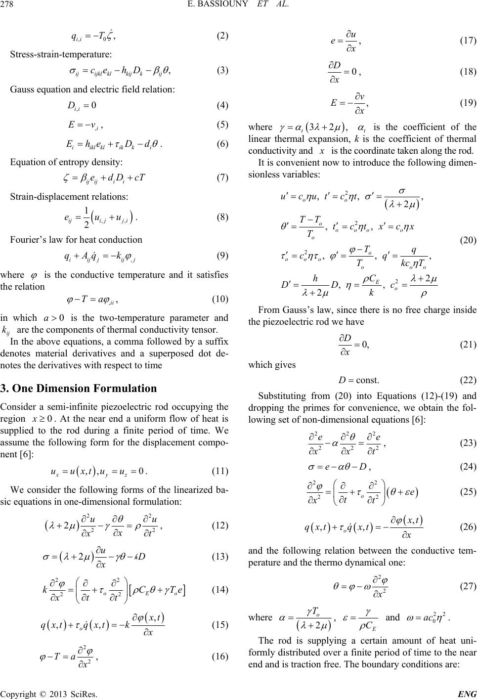

E. BASSIOUNY ET AL. 278
,0
,
ii
qT

  (2)
Stress-strain-temperature:
,
ijijkl klkijkij
ce hD

  (3)
Gauss equation and electric field relation:
,0 ii
D (4)
,i
Ev , (5)
iikl klikki
Ehe Dd

 . (6)
Equation of entropy density:
ij ijii
edDcT

 (7)
Strain-displacement relations:


,,
1
2
ijijj i
euu. (8)
Fourier’s law for heat conduction
,iijj ij
qAq kj


 (9)
where

is the conductive temperature and it satisfies
the relation
,ii
Ta

  , (10)
in which is the two-temperature parameter and
are the components of thermal conductivity tensor.
0a
ij
k
In the above equations, a comma followed by a suffix
denotes material derivatives and a superposed dot de-
notes the derivatives with respect to time
3. One Dimension Formulation
Consider a semi-infinite piezoelectric rod occupying the
region . At the near end a uniform flow of heat is
supplied to the rod during a finite period of time. We
assume the following form for the displacement compo-
nent [6]:
0x


,, 0
xy
uuxtuu
z

. (11)
We consider the following forms of the linearized ba-
sic equations in one-dimensional formulation:

22
2
2u
x2
u
x
t

 


 
, (12)

2uD
x


 

h
(13)

22
22
oE
kC
t xt



 



 o
Te (14)
 
,
,,
o
x
t
qxtqxt k
x





 (15)
2
2
Ta
x



, (16)
u
e
x



, (17)
0
D
x


, (18)
,
v
E
x



(19)
where


32,
t

  
t

is the coefficient of the
linear thermal expansion, k is the coefficient of thermal
conductivity and
x
is the coordinate taken along the rod.
It is convenient now to introduce the following dimen-
sionless variables:

2
2
2
2
,,,
2
,,
,,
2
,,
2
oo
o
ooo o
o
o
ooo
oo
E
o
ucutct
TT tctxcx
T
Tq
cq
TkcT
C
h
DD c
k





 

,
o






 
 






 



(20)
From Gauss’s law, since there is no free charge inside
the piezoelectric rod we have
0,
D
x


 (21)
which gives
const.D

(22)
Substituting from (20) into Equations (12)-(19) and
dropping the primes for convenience, we obtain the fol-
lowing set of non-dimensional equations [6]:
22
22
e
2
2
e
x
xt







, (23)
eD



, (24)

22
22
oe
t xt






 

 

(25)
 
,
,,
o
x
t
qxt qxt
x





 (26)
and the following relation between the conductive tem-
perature and the thermo dynamical one:
2
2
x



 (27)
where

2
o
T 



,
E
C

  and 22
0
ac

 .
The rod is supplying a certain amount of heat uni-
formly distributed over a finite period of time to the near
end and is traction free. The boundary conditions are:

E. BASSIOUNY ET AL. 279



,
o
ot
xs
F
t
x
 

 (28)
where o
F
is the heat flux intensity and


o
tt
 the
well-known impulse function:

10
0
o
o
o t
o
tt
t
t
tt








(29)
 
 
,0, ,0,0
,0,0,0,0
tet t
ttt


 
 
(30)
while the initial conditions are assumed to be:






,0 0,,0 0,,0 00xex xx    (31)
Applying the Laplace transform defined by:
   
0
e
st
Lftfsft t


d
(32)
to both sides of Equations (23)-(27), we obtain:
22
2
22
dd
dd
e
s
e
xx



, (33)
D
e
s
  , (34)

2
2
2
d,
do
2
o
s
sss
x

 e
(35)
  
,
1,
o
x
s
sq xs
x




, (36)
2
2
d,
d
x

  (37)
where s denotes the complex argument related to the
Laplace transform.
The transformed boundary conditions take the forms



1e
0, o
st
o
o
o
F
s
xts







(38)
Thus, the transformed component of the heat flux
vector becomes


0, 1
o
o
o
qs q
s




(39)
while the Equations (30) become



 
,0, ,0
,0, 0,0
tet
tt


 
 
,
,
(40)
and the corresponding transformed initial conditions of
the Equations (31) assume the form:






,0,0,0 00xex xx   
Eliminating

between Equations (35) and (37), we
get:
2
2
d
dLLe x


  , (42)
where


2
0
2
0
1
ss
LLs
s
s




 . (43)
Substituting from Equation (42) into Equation (37), we
obtain


1LLe

  . (44)
Using Equation (42) we can easily eliminate

be-
tween Equations (33) and (44) to obtain
2
2
d
d
e
M
Ne
x
  , (45)
where
 

 
2
1
1
1
1
LL
MMs L
s
LL
NNs L











(46)
Solving Equations (42) and (45) together we get the
following fourth order equation
42 0kakb





(47)
where, andaLN bLNLM


. It is worth men-
tioning here that the roots of Equation (47) are functions
of s and assume the forms:
22
12
44
,
22
aa baab
kk
 
 , (48)
where





  
11 1
11 1
oo o
o
ss ss
ass

 
 

  (49)


 

31
11 1
o
o
ss
bss




 

(50)
Thus the solutions of the Equations (42) and (45) sat-
isfying the boundary conditions at infinity are:
1
ee
2
x
kx
AB 


k
(51)
1
ee
2
x
k
eC D


xk
(52)
respectively, where 12 are the roots of the Equation
(47) and
,kk
,
A
B are parameters depending on s to be de-
termined using the boundary conditions while the rela-
tions between the coefficients ,, ,
A
BCD
are:

(41)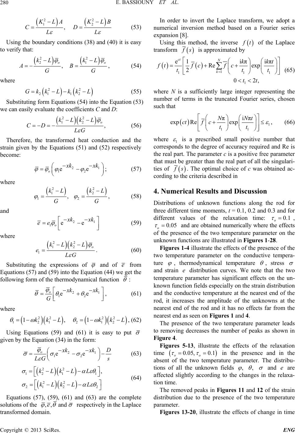

E. BASSIOUNY ET AL. 280
 
22
1
,
KLAKLB
CD
LL



2
(53)
Using the boundary conditions (38) and (40) it is easy
to verify that:




22
21
,
oo
kL kL
AB
GG

 
 , (54)
where



22
21 12
Gkk Lkk L (55)
Substituting form Equations (54) into the Equation (53)
we can easily evaluate the coefficients C and D:




22
12 , o
kLkL
CD LG



  (56)
Therefore, the transformed heat conduction and the
strain given by the Equations (51) and (52) respectively
become:
2
12
ee
o
1
x
kx
 





k
; (57)
where
 
22
1
12
,
kL kL
GG



2
, (58)
and
2
1ee o
1
x
kxk
ee 







(59)
where

22
12
1
o
kLkL
eLG



. (60)
Substituting the expressions of

and of e from
Equations (57) and (59) into the Equation (44) we get the
following form of the thermodynamical function

:
2
12
ee
o1
x
kx
G

 





k
, (61)
where








22 22
121212
1,1kkL kkL      , (62)
Using Equations (59) and (61) it is easy to put

given by the Equation (34) in the form:
21
12
ee
oD
xk xk
LG s









(63)





22
12 11
22
21 22
,kLkL L
kLkL L





 


 





(64)
Equations (57), (59), (61) and (63) are the complete
solutions of the ,, ande


In order to invert the Laplace transform, we adopt a
numerical inversion method based on a Fourier series
expansion [8].
Using this method, the inverse


f
t of the Laplace
transform


f
s is approximated by
 
1
11
1
e1 iπiπ
Re exp
2
02,
ct N
k
kk
ftfcf c
tt
tt
1
t
t



 

 






 (65)
where N is a sufficiently large integer representing the
number of terms in the truncated Fourier series, chosen
such that

1
11
πiπ
exp Reexp
NNt
ctf ctt





 



, (66)
where 1

is a prescribed small positive number that
corresponds to the degree of accuracy required and Re is
the real part. The parameter c is a positive free parameter
that must be greater than the real part of all the singulari-
ties of


f
s. The optimal choice of c was obtained ac-
cording to the criteria described in
4. Numerical Results and Discussion
Distributions of unknown functions along the rod for
three different time moments, t = 0.1, 0.2 and 0.3 and for
different values of the relaxation time: 0.1
o


,
0.05
o


and are obtained numerically where the effects
of the presence of the two temperature parameter on the
unknown functions are illustrated in Figures 1-28.
Figures 1-4 illustrate the effects of the presence of the
two temperature parameter on the conductive tempera-
ture

, thermodynamical temperature

, stress

and strain distribution curves. We note that the two
temperature parameter has significant effects on the un-
known function fields especially on the strain distribution
and the conductive temperature at the nearest end of the
rod, it increases the amplitude of the unknowns at the
nearest end of the rod and it has no effects far from the
nearest end as seen on Figures 1 and 4.
e
The presence of the two temperature parameter leads
to removing decreases the number of peaks as shown in
Figure 4.
Figures 5-13, illustrate the effects of the relaxation
time


0.05, 0.1
oo
 
in the presence and in the
absent of the two temperature parameter. The distribu-
tions of all the unknown fields ,

,


and are
affected slightly according to the changes in the relaxa-
tion time.
e
The removed peaks in Figures 11 and 12 of the strain
distribution due to the presence of the two temperature
parameter.
 respectively in the Laplace
transformed domain. Figures 13-20, illustrate the effects of change in time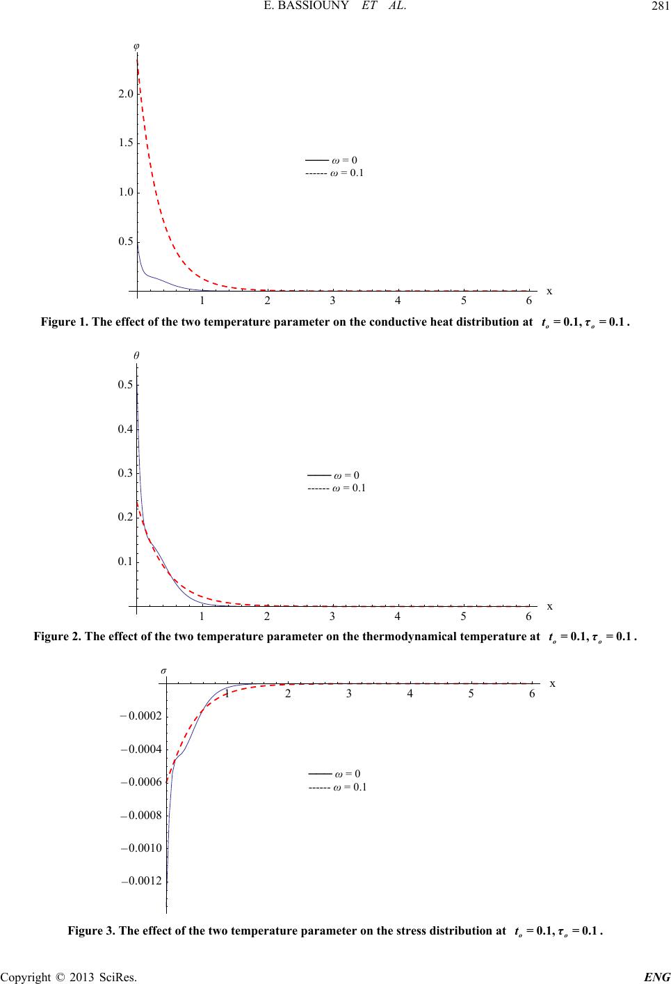

E. BASSIOUNY ET AL. 281
φ
___ 0
0.1
1 2 3 45 6x
0.5
1.0
1.5
2.0
─
── ω = 0
------ ω = 0.1
Figure 1. The effec t of the two tempera ture parameter on the conductive he at distribution at . =0.1, =0.1
oo
tτ
θ
___ 0
0.1
1
2
3
4
5
6
x
0.1
0.2
0.3
0.4
0.5
─
── ω = 0
------ ω = 0.1
Figure 2. The effect of the two temperature parameter on the thermodynamical temperature at .
=0.1, =0.1
oo
tτ
σ
___ 0
0.1
123456
x
0.0012
0.0010
0.0008
0.0006
0.0004
0.0002
─
── ω = 0
------ ω = 0.1
−
−
−
−
−
−
Figure 3. The effect of the two temperature parameter on the stress distribution at .
=0.1, =0.1
oo
tτ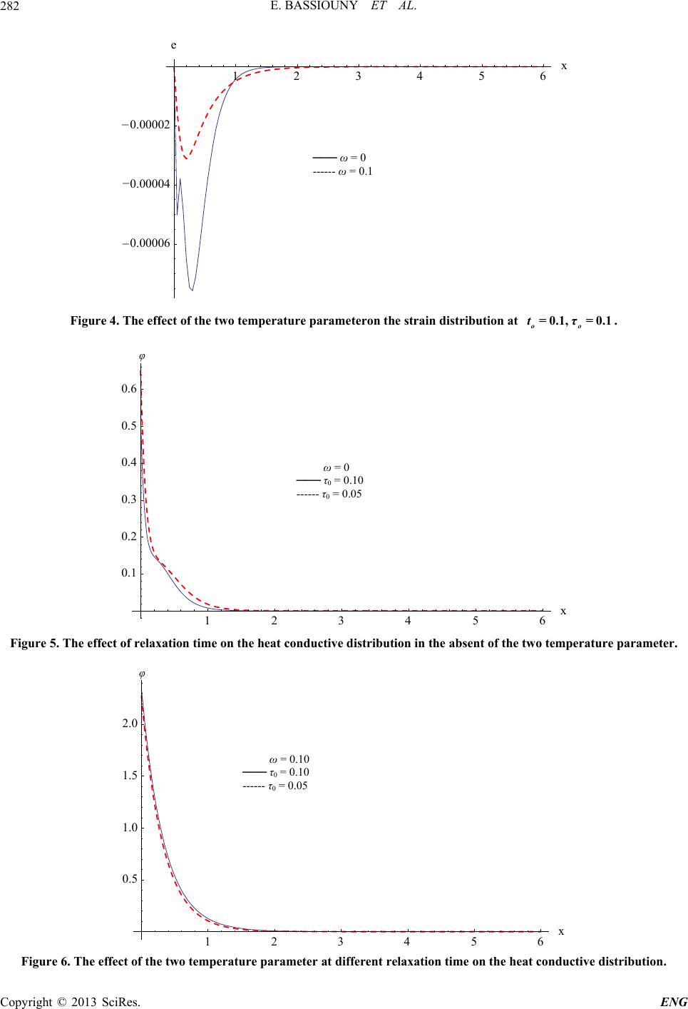

E. BASSIOUNY ET AL. 282
___ 0
0.1
1 23 45 6
x
0.00006
0.00004
0.00002
e
─
── ω = 0
------ ω = 0.1
−
−
−
Figure 4. The effect of the two temperature parameteron the strain distribution at . =0.1, =0.1
oo
tτ
φ
0
ــــــــــــــ 0 0.10
0 0.05
1 2 3 45 6x
0.1
0.2
0.3
0.4
0.5
0.6
ω = 0
─
── τ
0
= 0.10
------ τ
0
= 0.05
Figure 5. The effect of relaxation time on the heat conductive distribution in the absent of the two temperature parameter.
φ
0.10
ــــــــــــــ 0 0.10
0 0.05
1
2
3
4
5
6
x
0.5
1.0
1.5
2
.0
ω = 0.10
─
── τ0 = 0.10
------ τ0 = 0.05
Figure 6. The effect of the two temperature parameter at different relaxation time on the heat conductive distribution.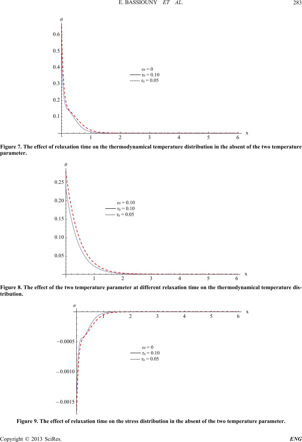

E. BASSIOUNY ET AL. 283
θ
0
ــــــــــــــ 0 0.10
0 0.05
1 2 3 45 6x
0.1
0.2
0.3
0.4
0.5
0.6
ω = 0
─
── τ
0
= 0.10
------ τ
0
= 0.05
Figure 7. The effect of relaxation time on the thermodynamical temperature distribution in the absent of the two temperature
parameter.
θ
0.10
ــــــــــــــ 0 0.10
0 0.05
1 23456
x
0
.05
0
.10
0
.15
0
.20
0
.25
ω = 0.10
─
── τ
0
= 0.10
------ τ
0
= 0.05
Figure 8. The effect of the two temperature parameter at different relaxation time on the thermodynamical temperature dis-
tribution.
σ
0
ــــــــــــــ 0 0.10
0 0.05
1 2 3 4 5 6x
0.0015
0.0010
0.0005
ω = 0
─
── τ
0
= 0.10
------ τ
0
= 0.05
−
−
−
Figure 9. The effect of relaxation time on the stress distribution in the absent of the two temperature parameter.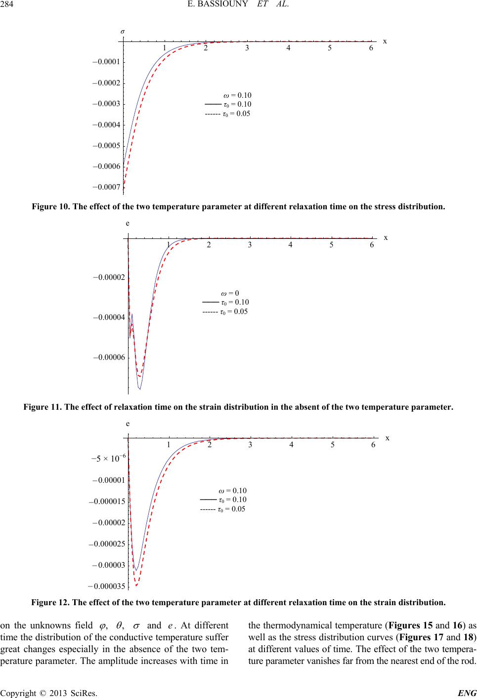

E. BASSIOUNY ET AL. 284
σ
0.10
ــــــــــــــ 0 0.10
0 0.05
1 2 3 4 5 6x
0.0007
0.0006
0.0005
0.0004
0.0003
0.0002
0.0001
ω = 0.10
─
── τ
0
= 0.10
------ τ
0
= 0.05
−
−
−
−
−
−
−
Figure 10. The effect of the two temperature parameter at different relaxation time on the stress distribution.
0
ــــــــــــــ 0 0.10
0 0.05
1 23 45 6x
0.00006
0.00004
0.00002
e
ω = 0
─
── τ
0
= 0.10
------ τ
0
= 0.05
−
−
−
Figure 11. The effect of relaxation time on the strain distribution in the absent of the two temperature parameter.
0.10
ــــــــــــــ 0 0.10
0 0.05
1 23 4 56
x
0.000035
0.00003
0.000025
0.00002
0.000015
0.00001
5. 10
6
e
ω = 0.10
─
── τ
0
= 0.10
------ τ
0
= 0.05
−
−
−
−
−
−
−5 × 10
−6
Figure 12. The effect of the two temperature parameter at different relaxation time on the strain distribution.
on the unknowns field ,

,


and . At different
time the distribution of the conductive temperature suffer
great changes especially in the absence of the two tem-
perature parameter. The amplitude increases with time in
the thermodynamical temperature (Figures 15 and 16) as
well as the stress distribution curves (Figures 17 and 18)
at different values of time. The effect of the two tempera-
ure parameter vanishes far from the nearest end of the rod.
e
t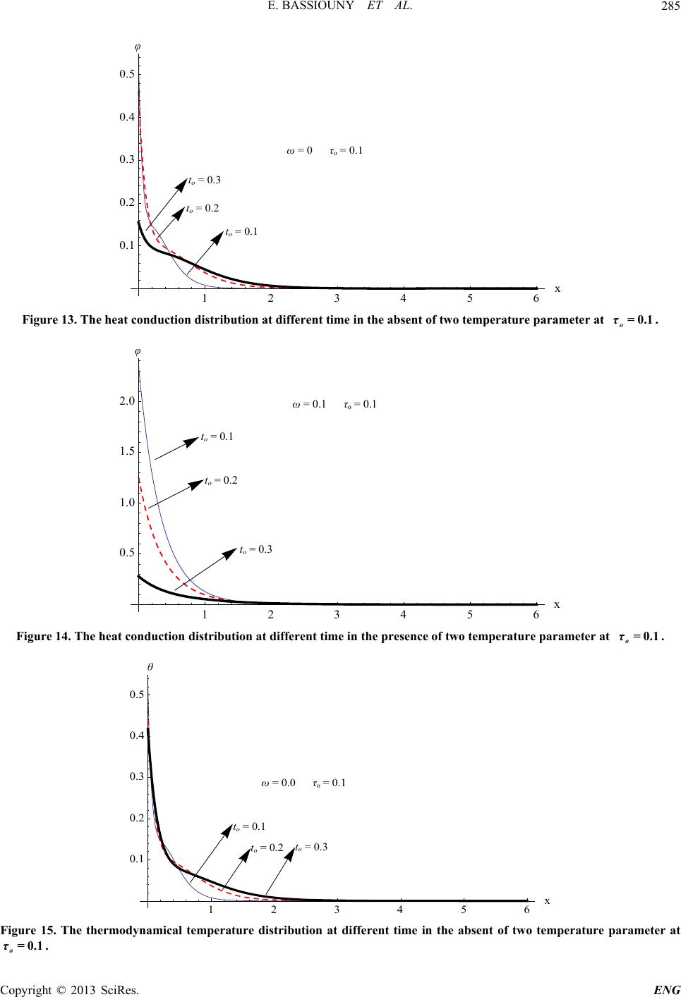

E. BASSIOUNY ET AL. 285
φ
=0.0
to=0.1
to=0.2
to= 0. 3
o=0.1
1 2 3 456x
0.1
0.2
0.3
0.4
0.5
t
o
= 0.1
ω = 0 τ
o
= 0.1
t
o
= 0.2
t
o
= 0.3
Figure 13. The heat conduction distribution at different time in the absent of two temperature parameter at . =0.1
o
τ
φ
=0.
to = 0.3
to=0 .2
to=0 .1
.1 o=0.1
1 2 3 456x
0.5
1.0
1.5
2
.0
t
o
= 0.1
ω = 0.1 τ
o
= 0.1
t
o
= 0.2
t
o
= 0.3
Figure 14. The heat conduction distribution at different time in the presence of two temperature parameter at . =0.1
o
τ
θ
to =0 .3
to=0.2
to =0 .1
=0.0 o=0.1
123456x
0.1
0.2
0.3
0.4
0.5
t
o
= 0.1
ω = 0.0 τ
o
= 0.1
t
o
= 0.2t
o
= 0.3
Figure 15. The thermodynamical temperature distribution at different time in the absent of two temperature parameter at
. =0.1
o
τ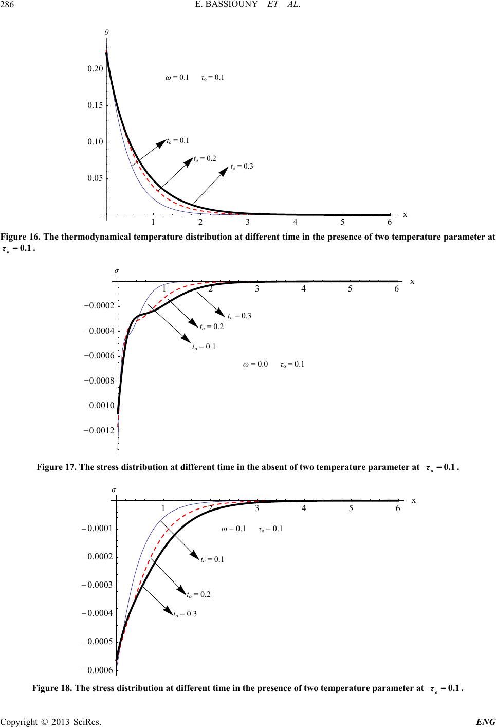

E. BASSIOUNY ET AL. 286
θ
to=0.3
to=0.2
to=0.1
=0.1 o=0.1
1 234 56x
0
.05
0
.10
0
.15
0
.20
t
o
= 0.1
ω = 0.1 τ
o
= 0.1
t
o
= 0.2
t
o
= 0.3
Figure 16. The thermodynamical temperature distribution at different time in the presence of two temperature parameter at
. =0.1
o
τ
σ
to =0.3
to =0.2
to =0.1
=0.0 o=0.1
1 2 3 4 5 6
x
0.0012
0.0010
0.0008
0.0006
0.0004
0.0002
t
o
= 0.1
ω = 0.0 τ
o
= 0.1
t
o
= 0.2
t
o
= 0.3
−
−
−
−
−
−
Figure 17. The stress distribution at different time in the absent of two temperature parameter at .
=0.1
o
τ
σ
=0.1
to= 0.1
to= 0.2
to= 0.3
o=0.1
123456x
0.0006
0.0005
0.0004
0.0003
0.0002
0.0001
t
o
= 0.1
ω = 0.1 τ
o
= 0.1
t
o
= 0.2
t
o
= 0.3
−
−
−
−
−
−
Figure 18. The stress distribution at different time in the presence of two temperature parameter at . =0.1
o
τ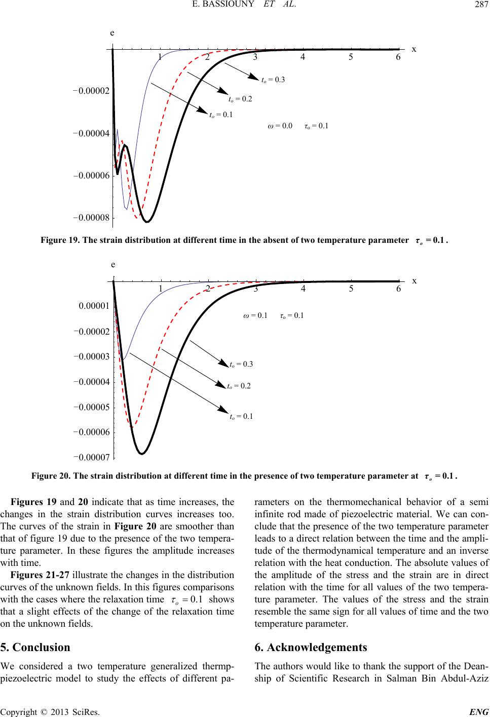

E. BASSIOUNY ET AL. 287
=0. 0
to = 0.3
to = 0.2
to=0 .1
o=0.1
1 2 3 45 6x
0.00008
0.00006
0.00004
0.00002
e
t
o
= 0.1
ω = 0.0 τ
o
= 0.1
t
o
= 0.2
t
o
= 0.3
−
−
−
−
Figure 19. The strain distribution at different time in the absent of two temperature parameter .
=0.1
o
τ
=0.1
to = 0 .2
to = 0 .3
o=0.1
to=0 .1
1 23 45 6x
0.00007
0.00006
0.00005
0.00004
0.00003
0.00002
0.00001
e
t
o
= 0.1
ω = 0.1 τ
o
= 0.1
t
o
= 0.2
t
o
= 0.3
−
−
−
−
−
−
Figure 20. The strain distribution at different time in the presence of two temperature parameter at . =0.1
o
τ
Figures 19 and 20 indicate that as time increases, the
changes in the strain distribution curves increases too.
The curves of the strain in Figure 20 are smoother than
that of figure 19 due to the presence of the two tempera-
ture parameter. In these figures the amplitude increases
with time.
Figures 21-27 illustrate the changes in the distribution
curves of the unknown fields. In this figures comparisons
with the cases where the relaxation time 0.1
o

 shows
that a slight effects of the change of the relaxation time
on the unknown fields.
5. Conclusion
We considered a two temperature generalized thermp-
piezoelectric model to study the effects of different pa-
rameters on the thermomechanical behavior of a semi
infinite rod made of piezoelectric material. We can con-
clude that the presence of the two temperature parameter
leads to a direct relation between the time and the ampli-
tude of the thermodynamical temperature and an inverse
relation with the heat conduction. The absolute values of
the amplitude of the stress and the strain are in direct
relation with the time for all values of the two tempera-
ture parameter. The values of the stress and the strain
resemble the same sign for all values of time and the two
temperature parameter.
6. Acknowledgements
The authors would like to thank the support of the Dean-
hip of Scientific Research in Salman Bin Abdul-Aziz s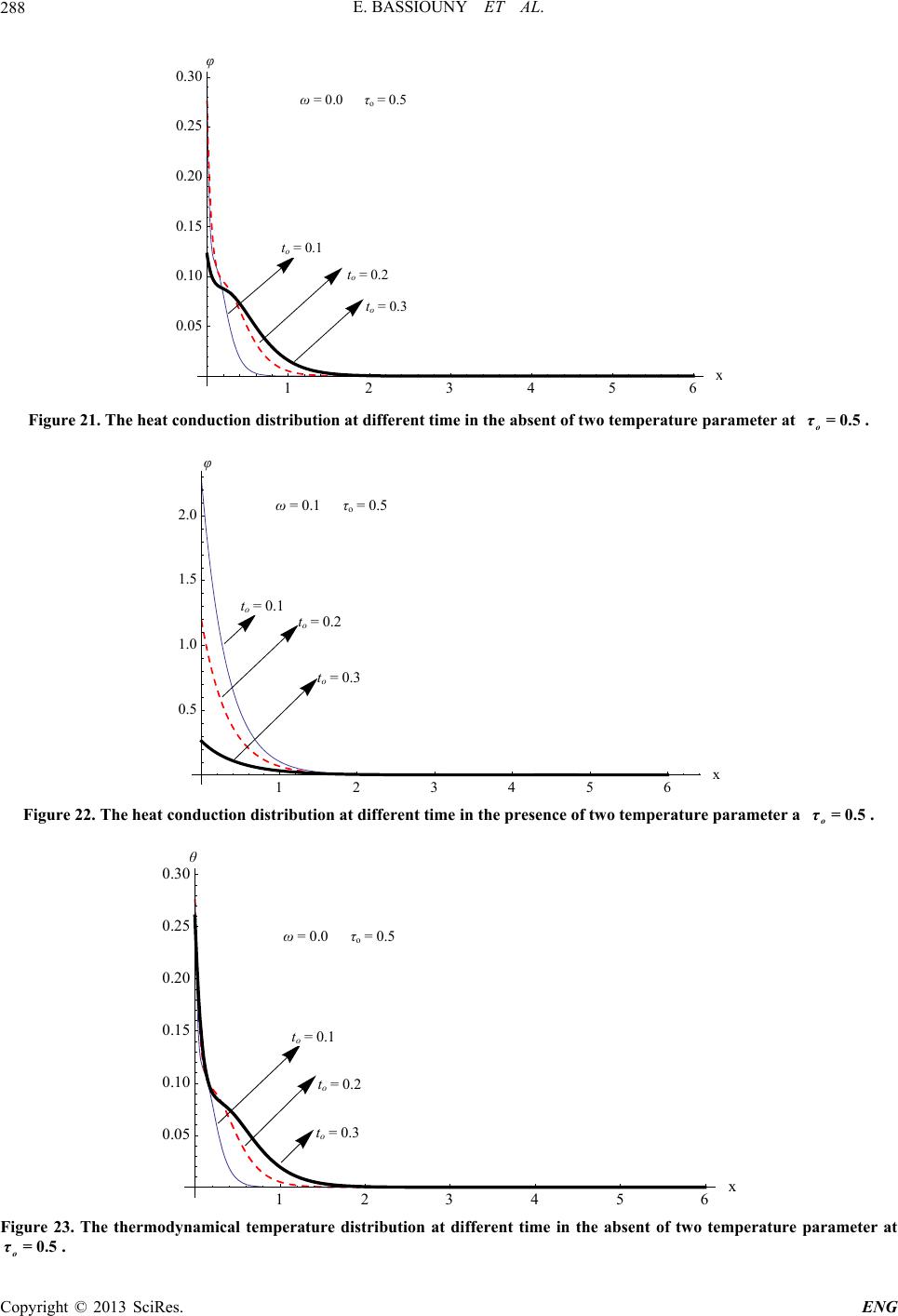

E. BASSIOUNY ET AL. 288
φ
=0.0 o=0.5
to=0.2
to=0.3
to=0.1
12 3 45 6
x
0.05
0.10
0.15
0.20
0.25
0.30
to = 0.1
ω = 0.0 τo = 0.5
to = 0.2
to = 0.3
Figure 21. The heat conduction distribution at different time in the absent of two temperature parameter at .
o
τ=0.5
φ
=0.1 o=0.5
to=0.1
to=0.2
to =0 .3
1 23 4 56x
0.5
1.0
1.5
2.0
t
o
= 0.1
ω = 0.1 τ
o
= 0.5
t
o
= 0.2
t
o
= 0.3
Figure 22. The heat conduction distribution at different time in the presence of two temperature parameter a .
o
τ=0.5
θ
=0.0 o=0.5
to=0.1
to=0.2
to=0.3
12 34 5 6
x
0.05
0.10
0.15
0.20
0.25
0.30
t
o
= 0.1
ω = 0.0 τ
o
= 0.5
t
o
= 0.2
t
o
= 0.3
Figure 23. The thermodynamical temperature distribution at different time in the absent of two temperature parameter at
.
o
τ=0.5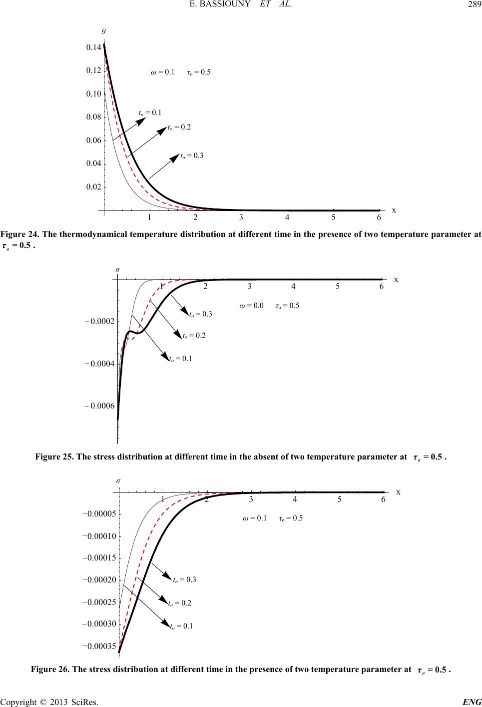

E. BASSIOUNY ET AL. 289
θ
=0.1 o=0.5
to=0.1
to=0.2
to=0.3
1 234 56
x
0.02
0.04
0.06
0.08
0.10
0.12
0.14
t
o
= 0.1
ω = 0.1 τ
o
= 0.5
t
o
= 0.2
t
o
= 0.3
Figure 24. The thermodynamical temperature distribution at different time in the presence of two temperature parameter at
.
o
τ=0.5
σ
=0.0 o=0.5
to=0. 1
to = 0.2
to= 0.3
1 2 3 4 5 6x
0.0006
0.0004
0.0002
t
o
= 0.1
ω = 0.0 τ
o
= 0.5
t
o
= 0.2
t
o
= 0.3
−
−
−
Figure 25. The stress distribution at different time in the absent of two temperature parameter at .
o
τ=0.5
σ
=0.1 o=0.5
to=0. 3
to=0. 2
to =0. 1
1 23 456
x
0.00035
0.00030
0.00025
0.00020
0.00015
0.00010
0.00005
t
o
= 0.1
ω = 0.1 τ
o
= 0.5
t
o
= 0.2
t
o
= 0.3
−
−
−
−
−
−
−
Figure 26. The stress distribution at different time in the presence of two temperature parameter at .
o
τ=0.5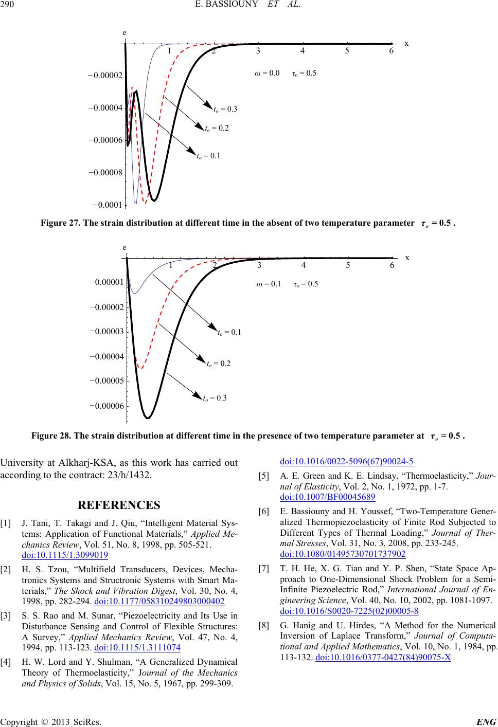

E. BASSIOUNY ET AL. 290
e
=0.0 o=0.5
to=0. 3
to = 0.2
to=0. 1
1 234 5 6x
0.0001
0.00008
0.00006
0.00004
0.00002
t
o
= 0.1
ω = 0.0 τ
o
= 0.5
t
o
= 0.2
t
o
= 0.3
−
−
−
−
−
Figure 27. The strain distribution at different time in the absent of two temperature parameter .
o
τ=0.5
e
=0.1 o=0.5
to=0.1
to=0.2
to=0.3
12 3 4 5 6x
0.00006
0.00005
0.00004
0.00003
0.00002
0.00001
t
o
= 0.1
ω = 0.1 τ
o
= 0.5
t
o
= 0.2
t
o
= 0.3
−
−
−
−
−
−
Figure 28. The strain distribution at different time in the presence of two temperature parameter at .
o
τ=0.5
University at Alkharj-KSA, as this work has carried out
according to the contract: 23/h/1432.
REFERENCES
[1] J. Tani, T. Takagi and J. Qiu, “Intelligent Material Sys-
tems: Application of Functional Materials,” Applied Me-
chanics Review, Vol. 51, No. 8, 1998, pp. 505-521.
doi:10.1115/1.3099019
[2] H. S. Tzou, “Multifield Transducers, Devices, Mecha-
tronics Systems and Structronic Systems with Smart Ma-
terials,” The Shock and Vibration Digest, Vol. 30, No. 4,
1998, pp. 282-294. doi:10.1177/058310249803000402
[3] S. S. Rao and M. Sunar, “Piezoelectricity and Its Use in
Disturbance Sensing and Control of Flexible Structures:
A Survey,” Applied Mechanics Review, Vol. 47, No. 4,
1994, pp. 113-123. doi:10.1115/1.3111074
[4] H. W. Lord and Y. Shulman, “A Generalized Dynamical
Theory of Thermoelasticity,” Journal of the Mechanics
and Physics of Solids, Vol. 15, No. 5, 1967, pp. 299-309.
doi:10.1016/0022-5096(67)90024-5
[5] A. E. Green and K. E. Lindsay, “Thermoelasticity,” Jour-
nal of Elasticity, Vol. 2, No. 1, 1972, pp. 1-7.
doi:10.1007/BF00045689
[6] E. Bassiouny and H. Youssef, “Two-Temperature Gener-
alized Thermopiezoelasticity of Finite Rod Subjected to
Different Types of Thermal Loading,” Journal of Ther-
mal Stresses, Vol. 31, No. 3, 2008, pp. 233-245.
doi:10.1080/01495730701737902
[7] T. H. He, X. G. Tian and Y. P. Shen, “State Space Ap-
proach to One-Dimensional Shock Problem for a Semi-
Infinite Piezoelectric Rod,” International Journal of En-
gineering Science, Vol. 40, No. 10, 2002, pp. 1081-1097.
doi:10.1016/S0020-7225(02)00005-8
[8] G. Hanig and U. Hirdes, “A Method for the Numerical
Inversion of Laplace Transform,” Journal of Computa-
tional and Applied Mathematics, Vol. 10, No. 1, 1984, pp.
113-132. doi:10.1016/0377-0427(84)90075-X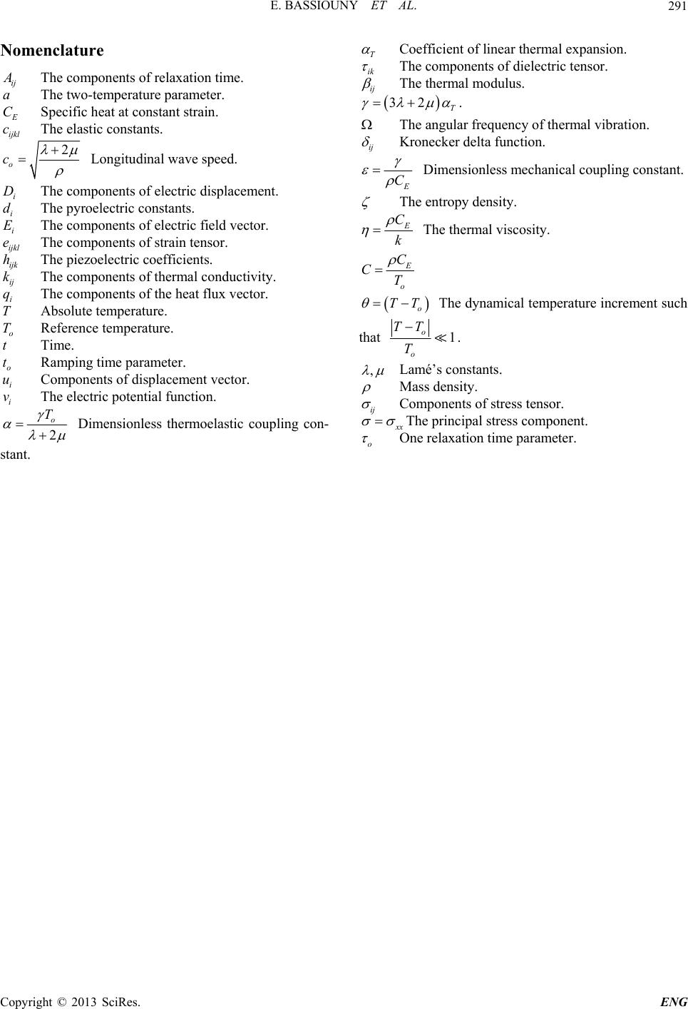

E. BASSIOUNY ET AL. 291
Nomenclature
ij
A
The components of relaxation time.
a The two-temperature parameter.
E
C
c
Specific heat at constant strain.
ijkl The elastic constants.
2
o
c




 Longitudinal wave speed.
i
D
d
The components of electric displacement.
i
E
The pyroelectric constants.
i
e
The components of electric field vector.
ijkl
h
The components of strain tensor.
ijk
k
The piezoelectric coefficients.
ij
q
The components of thermal conductivity.
i
T
The components of the heat flux vector.
Absolute temperature.
o
Time.
T
t
Reference temperature.
o
t
u
Ramping time parameter.
i
v
Components of displacement vector.
i The electric potential function.
2
o
T 



 Dimensionless thermoelastic coupling con-
stant.
T

Coefficient of linear thermal expansion.
ik

The components of dielectric tensor.
ij

The thermal modulus.


32 T

  .

The angular frequency of thermal vibration.
ij

Kronecker delta function.
E
C

  Dimensionless mechanical coupling constant.

The entropy density.
E
C
k

  The thermal viscosity.
E
o
C
CT




o
TT   The dynamical temperature increment such
that 1
o
o
TT
T
.
,

 Lamé’s constants.

Mass density.
ij

Components of stress tensor.
x
x



The principal stress component.
o

One relaxation time parameter.
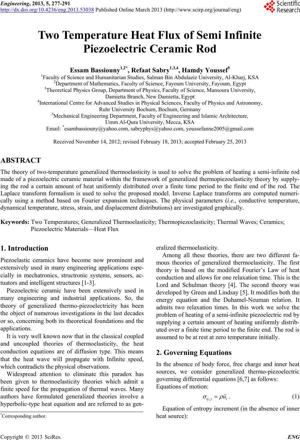