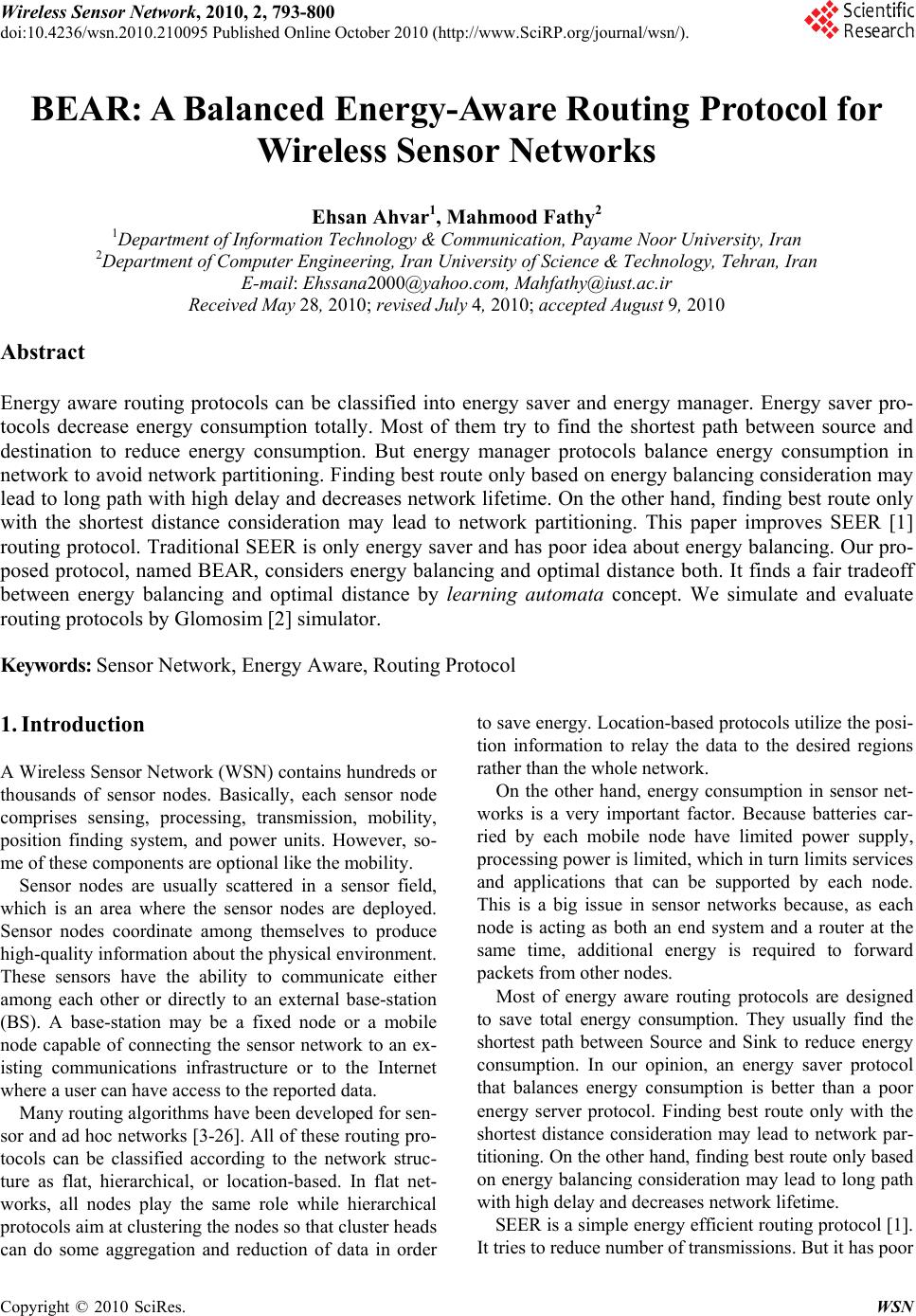Wireless Sensor Network, 2010, 2, 793-800
doi:10.4236/wsn.2010.210095 October 2010 (http://www.SciRP.org/journal/wsn/). Published Online
BEAR: A Balanced Energy-Aware Routing Protocol for
Wireless Sensor Networks
Ehsan Ahvar1, Mahmood Fathy2
1Department of Information Technology & Communication, Payame Noor University, Iran
2Department of Computer Engineering, Iran University of Science & Technology, Tehran, Iran
Received May 28, 2010; revised July 4, 2010; accepted August 9, 2010
Abstract
Energy aware routing protocols can be classified into energy saver and energy manager. Energy saver pro-
tocols decrease energy consumption totally. Most of them try to find the shortest path between source and
destination to reduce energy consumption. But energy manager protocols balance energy consumption in
network to avoid network partitioning. Finding best route only based on energy balancing consideration may
lead to long path with high delay and decreases network lifetime. On the other hand, finding best route only
with the shortest distance consideration may lead to network partitioning. This paper improves SEER [1]
routing protocol. Traditional SEER is only energy saver and has poor idea about energy balancing. Our pro-
posed protocol, named BEAR, considers energy balancing and optimal distance both. It finds a fair tradeoff
between energy balancing and optimal distance by learning automata concept. We simulate and evaluate
routing protocols by Glomosim [2] simulator.
Keywords: Sensor Network, Energy Aware, Routing Protocol
1. Introduction
A Wireless Sensor Network (WSN) contains hundreds or
thousands of sensor nodes. Basically, each sensor node
comprises sensing, processing, transmission, mobility,
position finding system, and power units. However, so-
me of these components are optional like the mobility.
Sensor nodes are usually scattered in a sensor field,
which is an area where the sensor nodes are deployed.
Sensor nodes coordinate among themselves to produce
high-quality information about the physical environment.
These sensors have the ability to communicate either
among each other or directly to an external base-station
(BS). A base-station may be a fixed node or a mobile
node capable of connecting the sensor network to an ex-
isting communications infrastructure or to the Internet
where a user can have access to the reported data.
Many routing algorithms have been developed for sen-
sor and ad hoc networks [3-26]. All of these routing pro-
tocols can be classified according to the network struc-
ture as flat, hierarchical, or location-based. In flat net-
works, all nodes play the same role while hierarchical
protocols aim at clustering the nodes so that cluster heads
can do some aggregation and reduction of data in order
to save energy. Location-based protocols utilize the posi-
tion information to relay the data to the desired regions
rather than the whole network.
On the other hand, energy consumption in sensor net-
works is a very important factor. Because batteries car-
ried by each mobile node have limited power supply,
processing power is limited, which in turn limits services
and applications that can be supported by each node.
This is a big issue in sensor networks because, as each
node is acting as both an end system and a router at the
same time, additional energy is required to forward
packets from other nodes.
Most of energy aware routing protocols are designed
to save total energy consumption. They usually find the
shortest path between Source and Sink to reduce energy
consumption. In our opinion, an energy saver protocol
that balances energy consumption is better than a poor
energy server protocol. Finding best route only with the
shortest distance consideration may lead to network par-
titioning. On the other hand, finding best route only based
on energy balancing consideration may lead to long path
with high delay and decreases network lifetime.
SEER is a simple energy efficient routing protocol [1].
It tries to reduce number of transmissions. But it has poor

E. AHVAR ET AL. 794
idea about energy management and energy balancing. On
the other hand, LABER routing protocol [20] tries to
balance energy consumption. But it has some visible
problems such as low accuracy in updating of energy and
high control overhead. In LABER, the Acknowledge-
ment packet is forwarded to previous data sender and the
other neighbors cannot update energy level of sender of
Acknowledgement; low accuracy. Moreover, the Ac-
knowledgment packet is an extra control overhead. We
try to update energy without Acknowledgment packets to
increase accuracy and decrease control overhead.
This paper addresses to design an energy-aware rout-
ing protocol for flat structure wireless sensor networks.
The proposed protocol, BEAR, tries to save and balance
energy consumption in network. It finds optimal route in
energy level and hop count both. Routing decisions in
BEAR are based on the distance to the Base Station as
well as on remaining battery energy levels of nodes on
the path towards the base station.
Section 2 discusses our design motivation and Section
3 presents SEER routing protocol. Section 4 discusses an
introduction about learning automata. In Section 5 we
present our proposed method. In Section 6 we present
simulation details and Section 7 presents the results. Sec-
tion 8 concludes on simulation results.
2. Motivation
Most of energy-aware routing protocols are only energy
saver. They do not have an acceptable idea about energy
balancing. This paper addresses to propose an energy
saver protocol that considers energy balancing too. We
found SEER routing protocol suitable to improve. SEER
routing protocol is a simple energy aware routing proto-
col that considers energy saving and energy balancing
both. But it has poor idea about energy balancing. Our
proposed routing protocol, named BEAR, improves SEER
in energy balancing and network lifetime.
3. SEER Routing Protocol
The different steps involved in the routing of packets in a
SEER network are discussed next. It is important to note
that each node is required to keep a neighbor table, which
contains an entry for each node within transmission dis-
tance.
STEP 1: Network setup and neighbor discovery
Once the network has been deployed in the area where
it is to operate, the sink transmits a broadcast packet. The
broadcast packet contains the header fields shown in Ta-
ble 1.
The source and destination addresses are 16 bit ad-
dresses enabling 65536 (216) unique addresses. Each no-
de in the network is assumed to have a unique address
Table 1. Fields contained in the network layer header of
broadcast messages.
Field Size (bits)
Source address 16
Destination address 16
Sequence number 8
Hop count 8
Energy level 16
Total 64
within the network. The 8-bit sequence number is used to
identify new broadcast messages. The sink increments the
sequence number every time it sends a new broadcast
message.
Nodes store the sequence number locally and forward
broadcast messages only if the sequence number of the
message is different from the stored one. The sequence
number uses 8 bits in order to ensure that latency in the
network does not cause nodes to mistakenly forward old
broadcast messages. An 8-bit hop count ensures that no-
des can be up to 255 hops from the sink.
When a node receives this initial broadcast message, it
checks whether it has an entry in its neighbor table for
the node that transmitted the message. If not, the receiver
node adds an entry that consists of the neighbor address,
hop count and energy level. The node then increments
the hop count stored in the message and stores this hop
count as its own hop count. It then retransmits the broad-
cast, but changes the source address field to its address
and the energy level field to its remaining energy level.
Every node in the network retransmits the broadcast me-
ssage once, to all of its neighbors.
If a node receives a broadcast message with a lower
hop count than the hop count it currently has, it updates
its hop count. When this initial broadcast has been flood-
ed through the network, each node knows its hop count
and has the address, hop count and energy level of each
of its neighbors.
STEP 2: Transmitting new data
When a node observes new data, as defined earlier, it
initiates the process of routing. Two types of data packets
can be sent: normal data and critical data. If a message is
considered critical, for example when the sensed tem-
perature changes from 25℃ to 100℃ within a very short
time, a flag is set in the message indicating that it is
critical. A node that originates a critical message trans-
mits it to two neighbors instead of only one. The fields
contained in the network layer header of data messages
are shown in Table 2.
The creator address field is used to inform the sink of
which node in the network originated the data message,
since the source address is changed at every hop of the
routing path. It is assumed that the sink knows where each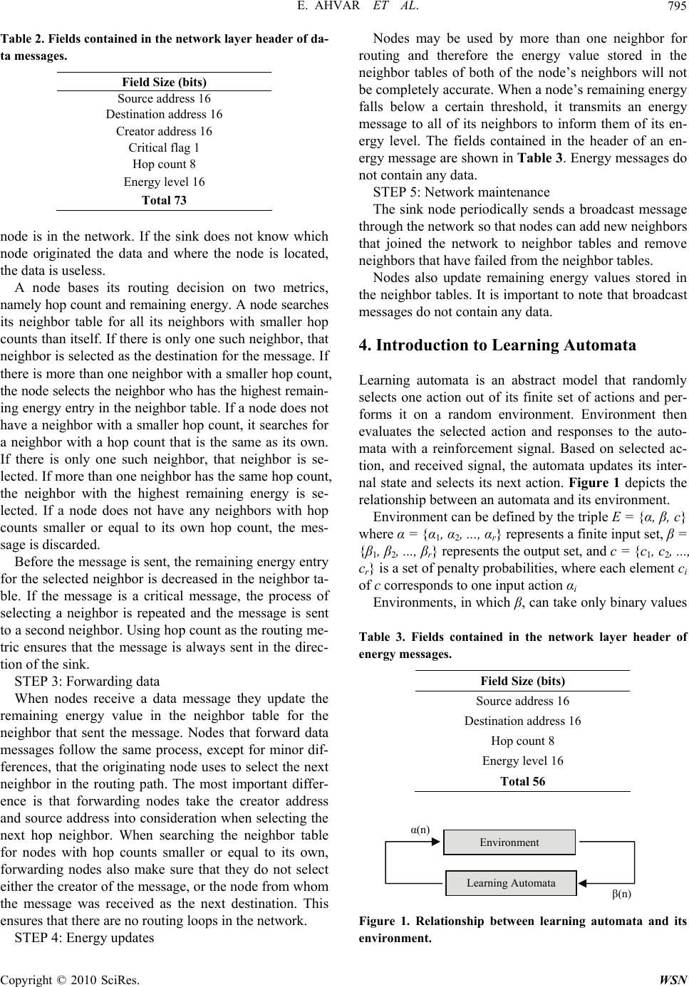

E. AHVAR ET AL. 795
Table 2. Fields contained in the network layer header of da-
ta messages.
Field Size (bits)
Source address 16
Destination address 16
Creator address 16
Critical flag 1
Hop count 8
Energy level 16
Total 73
(n)α
(n)β
Environmen
t
Learning Automata
node is in the network. If the sink does not know which
node originated the data and where the node is located,
the data is useless.
A node bases its routing decision on two metrics,
namely hop count and remaining energy. A node searches
its neighbor table for all its neighbors with smaller hop
counts than itself. If there is only one such neighbor, that
neighbor is selected as the destination for the message. If
there is more than one neighbor with a smaller hop count,
the node selects the neighbor who has the highest remain-
ing energy entry in the neighbor table. If a node does not
have a neighbor with a smaller hop count, it searches for
a neighbor with a hop count that is the same as its own.
If there is only one such neighbor, that neighbor is se-
lected. If more than one neighbor has the same hop count,
the neighbor with the highest remaining energy is se-
lected. If a node does not have any neighbors with hop
counts smaller or equal to its own hop count, the mes-
sage is discarded.
Before the message is sent, the remaining energy entry
for the selected neighbor is decreased in the neighbor ta-
ble. If the message is a critical message, the process of
selecting a neighbor is repeated and the message is sent
to a second neighbor. Using hop count as the routing me-
tric ensures that the message is always sent in the direc-
tion of the sink.
STEP 3: Forwarding data
When nodes receive a data message they update the
remaining energy value in the neighbor table for the
neighbor that sent the message. Nodes that forward data
messages follow the same process, except for minor dif-
ferences, that the originating node uses to select the next
neighbor in the routing path. The most important differ-
ence is that forwarding nodes take the creator address
and source address into consideration when selecting the
next hop neighbor. When searching the neighbor table
for nodes with hop counts smaller or equal to its own,
forwarding nodes also make sure that they do not select
either the creator of the message, or the node from whom
the message was received as the next destination. This
ensures that there are no routing loops in the network.
STEP 4: Energy updates
Nodes may be used by more than one neighbor for
routing and therefore the energy value stored in the
neighbor tables of both of the node’s neighbors will not
be completely accurate. When a node’s remaining energy
falls below a certain threshold, it transmits an energy
message to all of its neighbors to inform them of its en-
ergy level. The fields contained in the header of an en-
ergy message are shown in Table 3. Energy messages do
not contain any data.
STEP 5: Network maintenance
The sink node periodically sends a broadcast message
through the network so that nodes can add new neighbors
that joined the network to neighbor tables and remove
neighbors that have failed from the neighbor tables.
Nodes also update remaining energy values stored in
the neighbor tables. It is important to note that broadcast
messages do not contain any data.
4. Introduction to Learning Automata
Learning automata is an abstract model that randomly
selects one action out of its finite set of actions and per-
forms it on a random environment. Environment then
evaluates the selected action and responses to the auto-
mata with a reinforcement signal. Based on selected ac-
tion, and received signal, the automata updates its inter-
nal state and selects its next action. Figure 1 depicts the
relationship between an automata and its environment.
Environment can be defined by the triple E = {α, β, c}
where α = {α1, α2, ..., αr} represents a finite input set, β =
{β1, β2, ..., βr} represents the output set, and c = {c1, c2, ...,
cr} is a set of penalty probabilities, where each element ci
of c corresponds to one input action αi
Environments, in which β, can take only binary values
Table 3. Fields contained in the network layer header of
energy messages.
Field Size (bits)
Source address 16
Destination address 16
Hop count 8
Energy level 16
Total 56
Figure 1. Relationship between learning automata and its
environment.

E. AHVAR ET AL. 796
0 or 1 are referred to as P-models. A further generaliza-
tion of the environment allows finite output sets with
more than two elements that take values in the interval [0,
1]. Such an environment is referred to as Q-model. Fi-
nally, when the output of the environment is a continu-
ous random variable that assumes values in the interval
[0,1], it is referred to as an S-model. Learning automata
are classified into fixed-structure stochastic and variable
structure stochastic. In the following, we consider only
variable-structure automata.
A variable-structure automaton is defined by the qua-
druple {α, β, p, T} in which α = {α1, α2, …, αr } repre-
sents the action set of the automata, β = {β1, β2, …, βr}
represents the input set, p = {p1, p2, …, pr} represents the
action probability set, and finally p(n + 1) = T[α(n), β(n),
p(n)] represents the learning algorithm. This automaton
operates as follows. Based on the action probability set p,
automaton randomly selects an action αi , and performs it
on the environment. After receiving the environment's
reinforcement signal, automaton updates its action prob-
ability set based on Rel. (1) for favorable responses, and
Rel. (2) for unfavorable ones.
ijjnpanp
npanpnp
jj
iii


, )()1()1(
)](1[)()1(
(1)
ijjnpb
r
b
np
npbnp
jj
ii




)()1(
1
)1(
)()1()1( (2)
In these two equations, a and b are reward and penalty
parameters respectively. For a = b, learning algorithm is
called LR−P, for a << b, it is called LRεP, and for b = 0, it
is called LR−I. For more information about learning auto-
mat the reader may refer to [27].
5. BEAR Routing Protocol
BEAR is an extended version of traditional SEER rout-
ing protocol with some visible difference specially in for-
warding data procedure. The different steps involved in
the routing of packets in a BEAR network are discussed
next.
STEP 1: Network setup and neighbor discovery
The sink initializes the network by flooding the net-
work with a broadcast message. Each node that receives
the initiate packet adds an entry that consists of neighbor
id, energy level and hop count. Then it computes and in-
serts the selection probability of neighbor nodes into the
Neighbor List based on Rel. (3).
The node then increments the hop count stored in the
message and then retransmits the broadcast, but changes
the source address field to its address and the energy
level field to its remaining energy level. Every node in
the network retransmits the broadcast message only once,
to all of its neighbors.
When this initial broadcast has been flooded through
the network, each node knows their hop count, energy
level and probability of each of its neighbors.
11
Pr
1/
1/2 ()
1/
s
ss
mm
ii
ii
ob
HopCount EnergyLevel
s
m
HopCount EnergyLevel






(3)
STEP 2: Forwarding data
When a node observes new data it initiates the process
of routing. In traditional SEER, the neighbor with a hop
count that is smaller than the sending node’s hop count is
selected as the next hop. If multiple neighbors have
smaller hop counts, the neighbor with the highest re-
maining energy is selected as the next hop. If a node
does not have a neighbor with a smaller hop count, it
selects the neighbor with the highest remaining energy
from neighbors with an equal hop count to it. If the node
does not have a neighbor with an equal hop count to it,
the message is discarded.
But selecting next hop in our proposed protocol, BEAR,
is based on learning automata. A node searches into its
neighbor table for the neighbors with highest probability.
The energy level of data sender node is attached to ori-
ginal data packet, piggybacking. Then the data packet is
forwarded to neighbor with highest probability.
STEP 3: Updating energy and probabilities
All neighbors of data sender node receive the for-
warded data packet, by overhearing technique. They only
update the remaining energy value in the neighbor table
for the neighbor that sent the data packet, by piggyback-
ing technique, Figure 2(a). Also, the previous data sender
node receives its data packet again and updates all pro-
babilities in neighbor List, Figure 2(b).
In Figure 2(a), green node selects gray node as its
highest probability neighbor and forwards the data packet
to it. The gray node receives data packet and updates
energy level of green node in its Neighbor List. Another
neighbor only updates energy level of green node in their
Neighbor List and then discards the data packet. In Figure
Figure 2. Updating (a) energy level (b) energy level and
probabilities.
Data Sender
Next Select
Previous Data
Sender
Next Select
Data Sender

E. AHVAR ET AL.797
2(b), the gray node is data sender that selects the red
node as highest probability neighbor. Therefore, gray no-
de sends data to red. The red node receives the data pa-
cket from gray and update energy level of gray node.
Green node receives the data packet again by overhear-
ing and updates energy level of gray node and then up-
dates probability of its neighbors.
There are 4 behavioral scenarios when previous data
sender node receives the data packet by overhearing.
 If [(Energys/Avgenergy) + (HopCount/AvgHopCount)
< 2] then the route penalizes with β. β is computed based
on Rel. (6). (Very bad)
 If [(Energys/Avgenergy) + (HopCount/AvgHopCount)
= 2] then the route penalizes with β/2. (Bad)
 If [2 < (Energys/Avgenergy) + (HopCount/AvgHop-
Count) < 2.2] then the route rewards with α/2. α is com-
puted based on Rel. (5). (Acceptable)
 If [(Energys/Avgenergy) + (HopCount/AvgHopCount)
≥ 2] then the route rewards with α. α is computed based
on Rel. (5). (Good)
That Energys is the received energy of data sender no-
de, next selected node, and HopCount is the distance of
data sender node from Station.
Avgenergy is the average energy level of neighbor no-
des. AvgHopCount is average distance of all neighbor
nodes from the Station.
mlEnergyLeveAvgenergy
m
i
i/)(
1



(4)
In the Rel. (4), EnergyLeveli is the energy level of neigh-
bori and m is Neighbor List size.
Avghopcount is the average hopcounts of neighbor no-
des from the Station node.
mAvg
m
i
i/)HopCoun(HopCoun
1



(5)
In the Rel. (5), HopCounti is the distance of neighbori
from Station and m is Neighbor List size.
MaxHopInitEnergy
MaxEnergy ii


 HopCounHop
1

(6)
MaxHopAvgenergy
EnergyAvgenergy ii


HopCoun
2

(7)
In Rel. (6) and Rel. (7), α and β are reward and penalty
parameters respectively, HopCouni is distance between
sender node and Station node, In itEnergy is the initial
energy of nodes, Maxhop is maximum distance between
nodes in network and λ is minimum value for reward and
penalty parameters.
δ1 and δ2 are selected which cause to dose not exceed
of a threshold for α and β parameters.
The operation of the BEAR protocol can be summa-
rized as follows:
 The sink initializes the network by flooding the net-
work with a broadcast message.
 Nodes add all their neighbors’ information to their
neighbor tables.
 The node with highest probability is selected and
data packet is forwarded to it.
 The energy level of data sender node is updated by
its neighbors.
 The probability of data sender node is updated into
the Neighbor List of previous data sender node in each
hop.
BEAR routing protocol does not need an energy mes-
sage, Step.4 in traditional SEER, because the energy level
of each sender node is updated into its Neighbor Table
automatically, overhearing and piggybacking. Also the
sink node sends a broadcast message through the net-
work so that nodes can add new neighbors that joined the
network to neighbor tables and remove neighbors that
have failed from the neighbor tables. But sending rate of
broadcast message through the network is related to mo-
bility. The network with none mobility nodes dose no
need to send broadcast message as well as the network
with high mobility.
6. Simulation Model
This section simulates and compares our proposed rout-
ing protocol, BEAR, with traditional SEER routing pro-
tocol. To compare the routing protocols, a parallel dis-
crete event-driven simulator, GloMoSim, is used. Glo-
MoSim is a simulation tool for large wireless and wired
networks [2].
Table 4 describes the detailed setup for our simulator.
7. Simulation Results
In this section we evaluate and compare the various rout-
ing schemes. The performance measures of interest in this
Table 4. Simulation setting.
SIMULATION-TIME 1200 SECOND
TERRAIN-DIMENSIONS 1000 m * 1000 m
NUMBER-OF-NODES 200, 300, 500, 1000, 2000
NODE-PLACEMENT Uniform/Random
MOBILITY NONE
NUMBER OF EVENTS
(Sources) 100
TEMPARATURE 290.0 (in K)
RADIO-BANDWIDTH 2000000 (in bps)
RADIO-TX-POWER 5.0 (in dBm)
ENERGY- TRANSMIT-
LEVEL 0.0002 (in mW)
MAC-PROTOCOL 802.11
NETWORK-PROTOCOL IP
PROPAGA-
TION-PATHLOSS FREE-SPACE
RADIO-TYPE RADIO-ACCNOISE

E. AHVAR ET AL. 798
0
200
400
600
800
1000
1200
1400
200 300 50010002000
Nodes
Time[s]
SEER
BEAR
Figure 3. Time at which the first neighbor of Station fails
due to depleting its energy source. The nodes are randomly
distributed over the sensor area.
0
200
400
600
800
1000
1200
1400
2003005001000 2000
Nodes
Time[s]
SEER
BEAR
Figure 4. Time at which the first neighbor of Station fails
due to depleting its energy source. The nodes are uniformly
distributed over the sensor area.
0
50
100
150
200
2003005001000 2000
Nodes
Fails
SEER
BEAR
Figure 5. Number of fails at the end of simulation. The
nodes are randomly distributed over the sensor area.
0
50
100
150
200
250
2003005001000 2000
Nodes
Fails
SEER
BEAR
Figure 6. Number of fails at the end of simulation. The no-
des are uniformly distributed over the sensor area.
0
20
40
60
80
100
120
2003005001000 2000
Nodes
Actives(%)
SEER
BEAR
Figure 7. Percentage of active neighbors of Station at the
end of simulation. The nodes are randomly distributed over
the sensor area.
0
20
40
60
80
100
120
2003005001000 2000
Nodes
Actives(%)
SEER
BEAR
Figure 8. Percentage of active neighbors of Station at the
end of simulation. The nodes are uniformly distributed over
the sensor area.
0
0.00005
0.0001
0.00015
0.0002
20030050010002000
Nodes
Avg En
Consumption(mW)
SEER
BEAR
Figure 9. Average energy consumption (mW) in transmis-
sion mode. The nodes are randomly distributed over the
sensor area.
0
0.00005
0.0001
0.00015
0.0002
0.00025
2003005001000 2000
Nodes
Avg En
Consumption( mW)
SEER
BEAR
Figure 10. Average energy consumption (mW) in transmis-
sion mode. The nodes are uniformly distributed over the
sensor area.

E. AHVAR ET AL.799
study are: a) Average energy consumption of transmission
(in mW); b) Energy balancing. The variables are: number
of nodes and node placement.
The simulation of the protocols started with a broad-
cast message at the start of the simulation. We select 100
Sources to send data packets to the Station during the
simulation. The Sources are selected randomly in differ-
ent times. Each Source generates a 512-bit data packet
and forwards it through the network. Simulations are
performed to evaluate the network lifetime achieved by
each protocol. At the beginning of simulation, the trans-
mission energy level of each node was 0.0002 mW. Four
tests are achieved to evaluate the protocols:
Test 1: The time until the first neighbor of sink fails.
Test 2: Number of fails.
Test 3: Percentage of active neighbors of Station at the
end of simulation.
Test 4: The average remaining energy of all the nodes
in the network, at transmission mode.
Generally, the results from Test 1, Test 2, Test 3 and
Figures 3-8 show that BEAR is better than the SEER
protocol in energy managing. This is due to the fact that
BEAR sends data packet along a balanced path. Also at
the end of simulation BEAR has very low fails. There-
fore, performance of our protocol is very good especially
in high-density networks. On the other hand, the results
of Test 4, Figures 9 and 10 show that there are not visi-
ble difference in energy consumption between SEER and
BEAR.
Therefore, we could improve SEER routing protocol
in energy balancing without visible increment in energy
consumption. It means our BEAR routing protocol can
increase network lifetime compare with traditional SEER.
8. Conclusions
In this paper we studied energy aware routing protocols.
Then we proposed a new energy saver/balancer routing
protocol. The bease of our study was SEER routing pro-
tocol. We simulated and compared our routing protocol
with traditional SEER. Results showed that our protocol
generally was better than SEER in energy. Our BEAR
protocol had very low fails. It was more balancer than
SEER routing protocol especially in high-density net-
works. In general we found that BEAR gives better per-
formance, compared to SEER.
9. References
[1] G. P. Hancke and C. J. Leuschner, “SEER: A Simple
Energy Efficient Routing Protocol for Wireless Sensor Net-
works,” South African Computer Journal, Vol. 39, 2007,
pp. 17-24.
[2] X. Zeng, R. Bagrodia and M. Geria, “Glomosim: A Li-
brary for Parallel Simulation of Large Scale Wireless Net-
works,” Proceedings of the 12th Workshop on Parallel
and Distributed Simulations, Banff, 1998, pp. 154-161.
[3] M. Youssef, M. Younis and K. Arisha, “A Constrained
Shortest-Path Energy-Aware Routing Algorithm for Wire-
less Sensor Networks,” Proceedings of IEEE Wireless
Communications and Networking Conference, Orlando,
Vol. 2, 2002, pp. 794-799.
[4] D. Braginsky and D. Estrin, “Rumor Routing Algorithm
for Sensor Networks,” Proceeding of 1st ACM Workshop
on Sensor Networks and Applications, Atlanta, 2002, pp.
22- 31.
[5] T. Banka, G. Tandon and A. P. Jayasumana, “Zonal Ru-
mor Routing for Wireless Sensor Networks,” Proceedings
of IEEE Conference on Information Technology: Coding
and Computing, Las Vegas, Vol. 2, 2005, pp. 562-567.
[6] T. Hou, Y. Shi and J. Pan, “A Lifetime-Aware Single-
Session Flow Routing Algorithm for Energy-Constrained
Wireless Sensor Networks,” Proceedings of IEEE Mili-
tary Communications Conference, Boston, Vol. 1, 2003,
pp. 603-608.
[7] F. Block and C. Baum, “An Energy-Efficient Routing Pro-
tocol for Wireless Sensor Networks with Battery Level
Un- certainty,” Proceedings of IEEE Military Communi-
cations Conference, Anaheim, Vol. 1, 2002, pp. 489-494.
[8] A. Manjeshwar and D. P. Agrawal, “APTEEN: A Hybrid
Protocol for Efficient Routing and Comprehensive In-
formation Retrieval in Wireless Sensor Networks,” Pro-
ceedings of the 16th International Parallel and Distrib-
uted Processing Symposium, Fort Lauderdale, 2002, pp.
195-202.
[9] R. Manohar and A. Scaglione, “Power Optimal Routing in
Wireless Networks,” Proceedings of IEEE International
Conference on Communications, Seattle, Vol. 4, 2003, pp.
2979-2984.
[10] Z. W. Zheng, Z. H. Wu and H. Z. Lin, “Clustering Routing
Algorithm Using Game-Theoretic Techniques for WSNs,”
Proceedings of the International Symposium on Circuits
and Systems, Vancouver, Vol. 4, 2004, pp. IV-904-7.
[11] D. Petrovic, R. C. Shah, K. Ramchandran and J. Rabaey,
“Data Funneling: Routing with Aggregation and Com-
pression for Wireless Sensor Networks,” Proceedings of
the 1st IEEE International Workshop on Sensor Network
Protocols and Applications, Anchorage, 2003, pp. 156-162.
[12] C. Intanagonwiwat, R. Govindan and D. Estrin, “Directed
Diffusion: A Scalable and Robust Communication Para-
digm for Sensor Networks,” Mobile Networks and Ap-
plications, Vol. 1, No. 4, 2000, pp. 56-67.
[13] C. Chen, “Energy Efficient Routing for Clustered Wireless
Sensors Network,” Proceedings of the 29th Annual Con-
ference of the IEEE Industrial Electronics Society, Roa-
noke, Vol. 2, 2003, pp. 1437-1440.
[14] C. Schurgers and M. Srivastava, “Energy Efficient Rout-
ing in Wireless Sensor Networks,” Proceedings of IEEE
Military Communications Conference, Washington, Vol. 1,
2001, pp. 357-361.

E. AHVAR ET AL. 800
[15] M. Senouci and G. Pujolle, “Energy Efficient Routing in
Wireless Ad Hoc Networks,” Proceedings of IEEE In-
ternational Conference on Communications, Orlando, Vol.
7, 2004, pp. 4057-4061.
[16] D. Tian and N. Georganas, “Energy Efficient Routing with
Guaranteed Delivery in Wireless Sensor Networks,” Pro-
ceedings of IEEE Wireless Communications and Net-
working Conference, New Orleans, Vol. 3, 2003, pp. 1923-
1929.
[17] J. Zhang and H. Shi, “Energy-Efficient Routing for 2D
Grid Wireless Sensor Networks,” Proceedings of the In-
ternational Conference on Information Technology: Re-
search and Education, Newark, 2003, pp. 311-315.
[18] A. Datta, “Fault-Tolerant and Energy-Efficient Permuta-
tion Routing Protocol for Wireless Networks,” Proceed-
ings of the International Parallel and Distributed Proc-
essing Symposium, Nice, 2003, pp. 22-26.
[19] M. gholipour and M. R. Meybodi, “LA-Mobicast: A Learn-
ing Automata Based Distributed Protocol for Mobicast
in Sensor Networks,” Proceeding of 12th Annual Interna-
tional CSI Computer Conference, Tehran, 2007, pp. 1154-
1161.
[20] S. M. Abolhasani, M. R. Meybodi and M. Esnaashari, “LA-
BER: A Learning Automata Based Energy-Aware Routing
Protocol for Sensor Networks,” Proceedings of the 3rd
Information and Knowledge Technology, Ferdowsi Uni-
versity of Mashad, Mashad, 2007.
[21] Y. B. Ko and N. H. Vaidya, “Location-Aided Routing
(LAR) in Mobile Ad Hoc Networks,” Proceedings of the
IEEE International Conference on Mobile Computing and
Networking, Dallas, 1998, pp. 66-75.
[22] J. Broch, D. Johnson and D. Maltz, “The Dynamic Source
Routing Protocol for Mobile Ad Hoc Networks,” IETF
Internet Draft, 1999, work in progress. http://www.ietf.org/
internet-drafts/draft-ietfmanet-dsr-03.txt
[23] D. B. Johnson and D. A. Maltz, “Dynamic Source Routing
in Ad Hoc Wireless Networks,” Mobile Computing, Klu-
wer Academic Publishers, Vol. 353, 1996, pp. 153-181.
[24] C. E. Perkins and E. M. Royer, “Ad Hoc On-Demand
Distance Vector Routing,” Proceeding of the 2nd IEEE
Workshop on Mobile Computing Systems and Applica-
tions, New Orleans, 1999, pp. 90-100.
[25] T. He, J. Stankovic, C. Lu and T. Abdelzaher, “A Spatio-
temporal Communication Protocol for Wireless Sensor
Networks,” IEEE Transactions on Parallel and Distrib-
uted Systems, Vol. 16, No. 10, 2005, pp. 995-1006.
[26] Z. J. Haas and M. R. Pearlman, “The Zone Routing Pro-
tocol (ZRP) for Ad Hoc Networks,” IETF, MANET Inter-
net Draft, 1998.
[27] K. S. Narendra and M. A. L. Thathachar, “Learning Auto-
mata: An Introduction,” Prentice Hall, 1989.