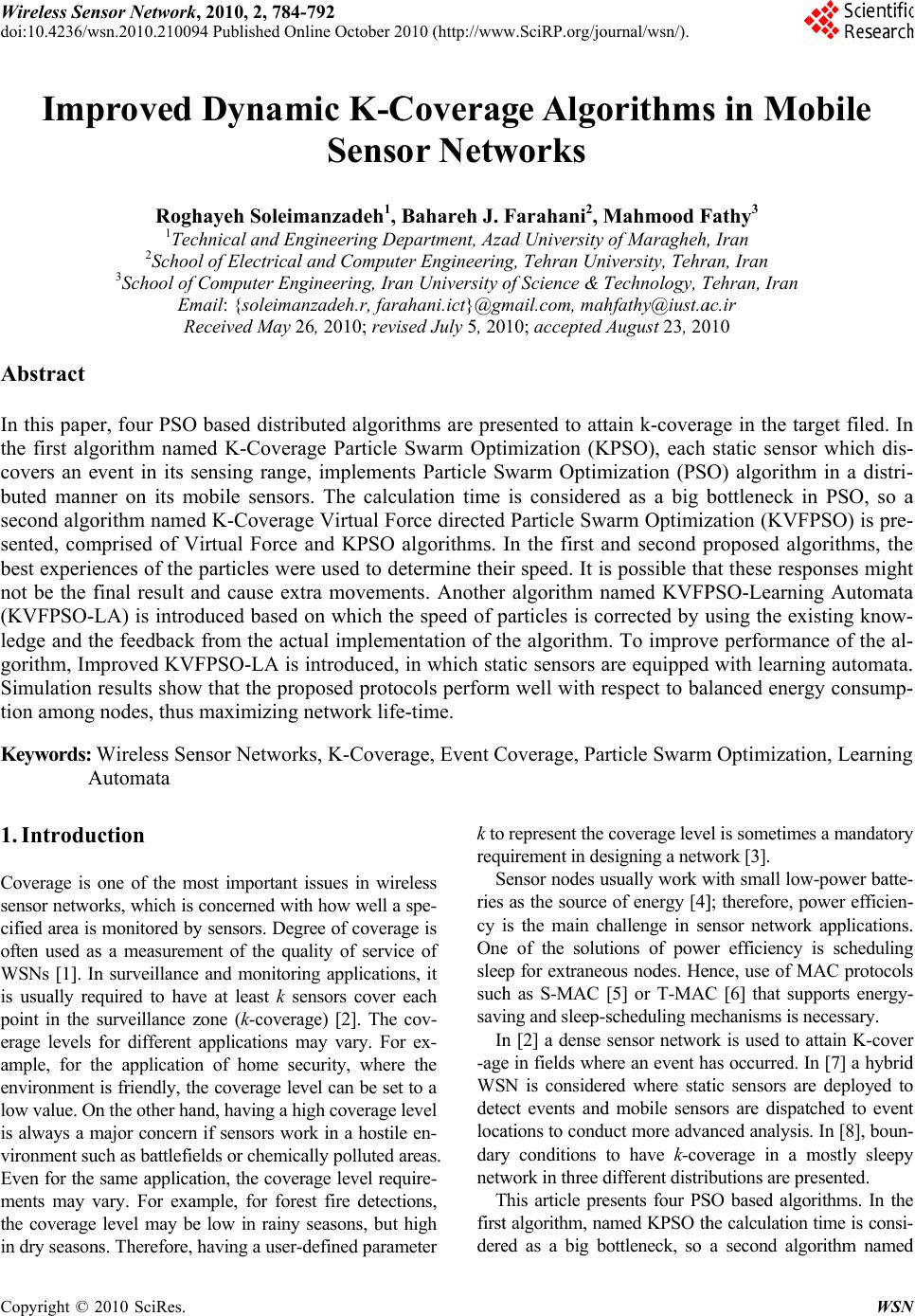Wireless Se
n
doi:10.4236/
w
Copyright ©
2
Im
p
Abstract
In this pap
e
the first al
g
covers an
e
b
uted man
n
second alg
o
sented, co
m
b
est experi
e
not be the
f
(KVFPSO-
L
ledge and t
h
gorithm, I
m
Simulation
tion among
Keywords:
W
A
1. Introdu
Coverage is
sensor netw
o
cified area is
often used a
s
WSNs [1]. I
n
is usually re
q
p
oint in the
erage levels
ample, for t
h
environment
low value. O
n
is always a
m
vironment s
u
Even for the
ments may
v
the coverage
in dry seaso
n
n
sor Network
,
w
sn.2010.2100
9
2
010 SciRes.
p
roved
Rog
h
1Tec
2Schoo
3School of
E
m
R
e
e
r, four PSO
g
orithm nam
e
vent in its s
n
er on its
m
o
rithm name
d
m
prised of
V
e
nces of the
f
inal result
a
L
A) is intro
d
h
e feedback
m
proved KV
F
results sho
w
nodes, thus
W
ireless Se
n
A
utomata
ction
one of the m
o
o
rks, which is
monitored
by
s
a measure
m
n
surveillance
q
uired to ha
v
surveillance
z
for different
h
e applicatio
n
is friendly, t
h
n
the other ha
n
m
ajor concern
u
ch as battlefi
e
same applica
t
v
ary. For exa
m
level may b
e
n
s. Therefore,
h
,
2010, 2, 784
9
4 Published O
n
Dyna
m
h
ayeh Solei
m
hnical and E
n
l of Electrica
l
Computer En
g
m
ail: {
s
oleim
a
e
ceived May
2
based distri
b
ed
K
-Cover
a
ensing rang
e
m
obile senso
r
d
K
-Covera
g
V
irtual Force
particles we
r
a
nd cause ex
d
uced based
from the ac
t
F
PSO-LA is
w
that the pr
o
maximizing
n
sor Networ
k
o
st important
concerned wi
t
y
sensors. De
g
m
ent of the q
u
and monitor
i
v
e at least k s
e
z
one (k-cover
a
applications
m
n
of home s
e
h
e coverage le
v
n
d, having a
h
if sensors w
o
e
lds or chemi
c
t
ion, the cove
r
m
ple, for for
e
e
low in rainy
h
aving a use
r
-
-792
n
line October 2
m
ic
K
-
C
Sens
o
m
anzadeh1,
B
n
gineering D
e
l
and Comput
e
g
ineering, Ir
a
a
nzadeh.
r
,
f
ar
a
2
6, 2010; revi
s
b
uted algori
t
a
ge Particle
e
, implemen
r
s. The calc
u
g
e Virtual F
o
and KPSO
r
e used to d
e
tra moveme
n
on which t
h
t
ual implem
e
introduced,
o
posed prot
o
network lif
e
k
s,
K
-Cover
a
issues in wir
e
t
h how well a
g
ree of covera
g
u
ality of servi
c
i
ng applicatio
n
e
nsors cover
a
ge) [2]. The
m
ay vary. Fo
r
e
curity, wher
e
v
el can be se
t
h
igh coverage
l
o
rk in a hostil
e
c
ally polluted
a
r
age level re
qu
e
st fire detect
i
seasons, but
-
defined para
m
010 (http://ww
w
C
overa
g
o
r Net
w
B
ahareh J.
e
partment, Az
a
e
r Engineerin
a
n University
o
a
hani.ic
t
m
s
ed July 5, 2
0
t
hms are pr
e
Swarm Opt
i
ts Particle S
u
lation time
o
rce directe
d
algorithms.
I
e
termine the
i
n
ts. Anothe
r
h
e speed of
p
e
ntation of t
h
in which st
a
o
cols perfor
m
e
-time.
a
ge, Event
C
e
less
spe-
g
e is
c
e of
n
s, it
each
cov-
r
ex-
e
the
t
to a
l
evel
e
en-
a
reas.
qu
ire-
i
ons,
high
m
eter
k to
req
u
S
ries
cy
i
On
e
sle
e
suc
h
sav
i
I
n
-ag
e
W
S
det
e
loc
a
dar
y
net
w
T
firs
t
der
e
w
.SciRP.org/j
o
g
e Alg
o
w
orks
Farahani2,
M
a
d University
g, Tehran Un
o
f Science &
T
m
ail.com, ma
h
0
10; accepted
A
e
sented to at
t
i
mization (
K
warm Opti
m
is consider
e
d
Particle S
w
I
n the first
a
ir
speed. It i
s
r
algorithm
n
p
articles is c
o
h
e algorith
m
a
tic sensors
a
m
well with
r
C
overage, Pa
r
represent the
u
irement in d
e
S
ensor nodes
u
as the sourc
e
i
s the main c
h
e
of the solu
t
e
p for extrane
o
h
as S-MAC
i
ng and sleep-
n
[2] a dense
e
in fields wh
e
S
N is conside
r
e
ct events an
d
a
tions to cond
u
y
conditions
w
ork in three
d
T
his article pr
e
t
algo
r
ithm, n
a
e
d as a big b
o
urnal/wsn/).
o
rithm
s
M
ahmood
F
of Maragheh
,
iversity, Tehr
a
T
echnology,
T
h
a
A
ugus
t
23, 2
0
t
ain k-cover
a
K
PSO), each
m
ization (PS
O
e
d as a big
b
w
arm Optimi
z
a
nd second
p
s
possible t
h
n
amed KVF
P
o
rrected by
u
m
. To impro
v
a
re equippe
d
r
espect to b
a
r
ticle Swar
m
coverage lev
e
e
signing a net
w
u
sually work
w
e
of energy [4
]
h
allenge in s
e
t
ions of pow
e
o
us nodes. H
e
[5] or T-MA
C
scheduling m
e
sensor netwo
r
e
re an event
h
r
ed where sta
t
d
mobile sens
o
u
ct more adv
a
to have k-co
v
d
ifferent distr
i
e
sents four P
S
a
med KPSO t
h
ottleneck, so
s
in M
o
F
athy3
,
Iran
a
n, Iran
T
ehran, Iran
a
c.i
r
0
10
a
ge in the ta
r
static senso
O) algorith
m
b
ottleneck i
n
z
ation (KVF
p
roposed al
g
h
at these res
p
P
SO-Learni
n
u
sing the ex
i
v
e performa
n
d
with learni
n
a
lanced ener
g
m
Optimizati
o
e
l is sometime
w
ork [3].
w
ith small lo
w
]
; therefore, p
o
e
nsor networ
k
e
r efficiency
e
nce, use of
M
C
[6] that su
p
e
chanisms is
n
r
k is used to
a
h
as occurred.
I
t
ic sensors ar
e
o
rs are
d
ispa
t
a
nced analysis
v
erage in a
m
i
butions are p
r
S
O based alg
o
h
e calculation
a second alg
o
WS
N
o
bile
r
get filed. I
n
r which dis
-
m
in a dist
r
i
-
n
PSO, so
a
PSO) is p
r
e
-
g
orithms, th
e
p
onses migh
t
n
g Automat
a
i
sting know
-
n
ce of the al
-
n
g automata
.
g
y consump
-
o
n, Learnin
g
s a mandator
y
w
-power batte
-
o
wer efficien
-
k
applications
.
is schedulin
g
M
AC protocol
s
p
ports energ
y
-
n
ecessary.
a
ttain K-cove
r
I
n [7] a hybri
d
e
deployed t
o
t
ched to even
t
. In [8], boun
-
m
ostly sleep
y
r
esented.
o
rithms. In th
e
time is consi
-
o
rithm name
d
N
n
-
-
a
-
e
t
a
-
-
.
-
g
y
-
-
.
g
s
-
r
d
o
t
-
y
e
-
d

R. SOLEIMANZADEH ET AL. 785
KVFPSO is presented comprised of Virtual Force and KP-
SO algorithms and as the result, less energy is consumed.
The other algorithm named KVFPSO-LA is intro-
duced, based on which the speed of particles is corrected
by using the existing knowledge and the feedback from
the actual implementation of the algorithm, in addition to
using the law of virtual force. In this method, there will
be less movement and re-location to achieve the desired
result. Finally a new algorithm named Improved KVFPSO-
LA is introduced, in which static sensors are equipped
with learning automata. As the result, only the required
numbers of mobile nodes are re-located.
2. System Model
In this paper, a mobile sensor network is a collection of
the mobile nodes, which have mobility and are able to
change their position based on networks dynamics or
requirements. The system model is as followings:
 Mobile sensors are aware of their location by using
locating algorithms [9].
 1-coverage is set up by using the method mentioned
in [10] with minimum number of sensors and using the
least amount of energy in the concerned field. All mobile
sensors used for 1-coverage will be mentioned as static
sensors.
 The communication range of sensors is greater or
equal to their sensing range. As the result, static sensors
are connected to each other. (Rc > = 2Rs)
 Covering detection model in these algorithms is Bi-
nary Detection Model [11].
 Static sensors use to detect an event that has oc-
curred in their sensing range and determine a coverage
degree, based on the size of the event and environmental
situations [3]. Then, based on the methods, which will be
discussed later, they would increase coverage degree for
that event to a determined extent.
 These protocols consist of five phases:
1-Initialization Phase, 2-Proxy Sensor Selection Phase,
3-Creating Mobile Sensor List Phase, 4-Creating Par-
ticle List Phase, 5-Running the Algorithm Phase
Phases 1-4 are in common within all proposed algo-
rithms and only the last phase varies, which will be dis-
cussed in herewith.
3. Algorithms Implementation Phases
3.1. Initialization Phase
In this phase, all mobile sensors would broadcast one hello
message in the network. Static sensors in their commu-
nication range, which have received this message which
would in response, create and send a feedback message
consisting of two fields: identification number of static
sensor and the location of the static sensor.
3.2. BProxy Sensor Selection Phase
In this phase, the mobile sensors should select one among
many static sensors, which have sent feedback message
to them. Therefore, a proxization probability is determined
for each static sensor, which will be calculated using Equ-
ation (1). Then, the mobile sensor will choose as its pro-
xy the static sensor, which has the highest probability. If
more than one sensor has equal probability, the proxy
selection will be done based on order of receiving me-
ssages, sending to it a delegate proxy request consisting
of three fields. These would include the mobile iden-
tification number, level of remaining energy and the lo-
cation where in these fields are initialized in sequence
with mobile sensor Mac address, mobile energy level and
its location. From there on, all relocations of mobile sen-
sors shall be done under their proxy sensors.

1
1/
m
ii
i
Pad d

 
dThedistance betweenproxy

(1)
i
node aandthe mobilenode
In this equation, m refers to the number of static sen-
sors which have sent a feedback message for the mobile.
The distance between the static sensor and the mobile is
calculated by using the Euclidean distance.
After all mobile sensors have selected a proxy for
themselves; they go to the sleep mode to cut down on
energy consumption using the method mentioned in [5]
and [6]. If an event occurs in their proxy’s sensing area
or if selected as appropriate for relocating, as per a re-
quest of other static sensors from its proxy, its proxy will
wake it up by sending an awakening message to it.
3.3. Creating Mobile Sensor List Phase
This phase will be started by any static node, which de-
tects an event in its sensing range. When the static sensor
detects an intruder in its sensing range, it will determine
how many mobile sensors are needed according to the
size and bigness of the intruder and environmental situa-
tions; meaning that in this phase it calculates the size of
K. For example, it can be said that K is a coefficient of
the size of the intruder, for instance it needs five mobile
sensors (6-coverage) for a panzer and two extraneous
mobile sensors (3-coverage) for a soldier.
After determining the size of K, the proxy sensor which
has detected an event in its sensing range refers to mo-
biles sensors which represent them and evaluates wheth-
er it has enough number of mobile sensors. In this phase,
the following might happen for the static sensor:

786 R. SOLEIMANZADEH ET AL.
If the number of its mobile sensors is greater or equal
to K, those of its sensors with less distance, compared to
the sensing range with the event, are awakened with a
message. The other sensors are put in a list named the list
of mobile sensors and advances to the next phase.
Otherwise, the following might occur:
If the number of mobile sensors is less than K, like the
previous phase, those of its sensors which have less dis-
tance than the sensing range to the event are awakened
and the other sensors are put in the list of mobile sensors.
It would then assess the degree of coverage, deduct it
from K, and the final amount will determine the number
of mobiles which should be taken from the neighbors.
Subsequently, it would send a message of request to its
neighboring static sensors, which would include ID num-
ber of the static sensor (proxy) and location of the event.
The adjacent static sensors which receive the message
would evaluate it and might undertake either of the fol-
lowing actions:
 If, there is no event in its sensing range and has no
need for its mobile sensors, in a message to static sensor,
the mobile requester would send the list of mobiles. This
message would include its own ID number as well as that
of its other mobiles and the location of its mobiles and
the level of energy.
 If the neighboring sensor has also detected an event
and its mobile sensors are engaged, then even if it has
extraneous mobiles (i.e. the number of its mobiles are
more than the number of K), it would give a negative
reply to the requesting proxy. This is because there is the
possibility that it again detects an event in the near future
in its sensing range and might need its mobiles.
The requesting static sensor, given the amount of K,
gives a positive response to those static sensors, which
fulfill its need. Therefore, it takes the specifications of its
mobile sensors and puts them in the list of mobile sen-
sors. Thus, a list, including mobile sensors on which
algorithm will be implemented, is created.
3.4. Creating Particle List Phase
Each static sensor, which has discovered an event in its
sensing range, starts this phase after creating a list of
mobile sensors, creating its particle list. In this section, a
record will be attributed to each sensor existing in the
mobile sensors’ list, which would include ID fields, loca-
tion and energy level of the mobile sensor. At the same
time, an initial speed is by coincidence attributed to it.
3.5. Running the Algorithm Phase
3.5.1. K-C overage Particl e Sw arm Op ti mization
(KPSO) Algorithm
This algorithm is implemented in distributed form by
static sensors, which have detected an event in their sen-
sing range. In this algorithm, each static sensor, which de-
tects an event in its sensing range, implements 1-4 phas-
es and thus, creates its particle list. Then, it implements
the PSO algorithm on its particles [11]. In this algorithm,
the function fitness will be the distance between the mo-
biles and the location of the event. Implementing this
algorithm will continue until maximum number of repe-
tition is achieved or the determined degree of coverage is
attained by the proxy sensors for the event.
3.5.2. K-Coverage Virtual Force Directed Particle
Swarm Optimization (KVFPSO) Algorithm
In KPSO algorithm, although the desired result is achi-
eved, but the calculation time in this algorithm is a big
bottleneck. Also, the speed of particles in this algorithm
is determined only by using the local and global best
experiences. This is while, there is the possibility that
these might not be the best final results and cause extra
and repeated movements.
To counter this problem, the law of virtual force has
been used to determine the speed of particles in this al-
gorithm. To do this, the locations of events are consi-
dered regions with preferred coverage area and in a cir-
cular shape. (Regions with preferred coverage area are
regions where mobile sensors are attracted towards these
regions by a force of attraction). The center of the circle is
presumed as the location of the event and the radius of
the circle is presumed as the sensing range of the sensors.
Regions with preferred coverage are shown with Am and
the force of attraction applied to the sensor moving to-
wards the location of the event is calculated as the fol-
lowing [11]:


,
0
Apre AmiAmiAmAm
iAm
WPifrdr C
F
otherwise







(2)
where r and c are the sensing range and communication
range of mobile sensors. rAm and pAm are the radius and
importance level parameter of the area of preferential
coverage Am , wApre is a measure of the attractive forces
exerted by obstacles , diAm is the distance between si and
Am, αiAm is the orientation of a line segment from si to Am.
KVFPSO algorithm also is a distributed algorithm wh-
ich is implemented by any static sensor which has detected
an event in its sensing range. In this algorithm, the follow-
ing equation is used to determine the speed of particles:
vij (t + 1) = w(t)* vij(t)
+ c1 * r1i(t) *(pbestij(t) – positionij(t))
+ c2 * r2i(t)* (gbestij(t) – positionij(t))
+ c3*r3i(t)*gij(t) (3)
where vij(t) and positionij(t) represent the position and
velocity of ith particle in the jth dimension at time t.
pbestij(t) is the local best position of ith particle in jth

R. SOLEIMANZADEH ET AL. 787
dimension and gbestij(t) is the global best position. r1i(t)
and r2i(t) are two separate random function in the range
[0,1]. c1, c2 are learning factors. The velocity of particle
in each dimension is limited to the Vmax[i] which i is the
index of dimension. c3 is acceleration constant, r3i(t) is
also a random function in the range [0,1] which is inde-
pendent to r1i(t) and r2i(t), gij(t) is the prolepsis motion
suggested by virtual force of ith particle in jth dimension
[11] , which is computed by:



1
(, 2)
(, 2)
1
1
(, 2)
1
(, 2)
1
(, 2)
(, 2)
()
j
i
xy
j
i
xy
j
i
F
x
j
i
xy
ij j
i
F y
j
i
xy
F
M
axStep ejodd
F
gt
F
M
axStep ejeven
F






 









(4)
where the superscript of each parameter presents the in-
dex of particles and the index of wireless sensor nodes
which the virtual force exerts on, the subscript presents
the coordinate of the virtual force. The correlative virtual
forces are carried out by Equation (2).
In this algorithm, in addition to using the local best
experience and the global best experience, the law of
virtual force is also used to determine the speed of the
particles. Adding this force to the speed of particles cau-
ses them to move towards the location of the event at a
faster pace. As the result, the algorithm achieves result
with less number of repetitions and mobiles move more
objectively. Therefore, in this method, there will be less
re-location to achieve the desired result, causing less ener-
gy consumption.
3.5.3. K-Coverage Virtual Force Directed Particle
Swarm Optimization - Learning Automata
(KVFPSO-LA) Algorithm
In the standard PSO algorithm, the responsibility to strike
a balance between global and local search is with the me-
dian coefficient. This coefficient determines how much of
the particle’s current speed was used in determining its
speed in the next phase. However, in [12], a new algo-
rithm has been recommended which uses learning auto-
mata to regulate the method of searching for particles. It
is the learning automata which determine in each step
that particles continue in their current route or follow the
best particles found so far. Using the learning automata
has two advantages: First, the existing knowledge can be
used to determine the trend of changes in the medial
weight, and second, the trend can be corrected in the ac-
tual environment by using the feedback from implemen-
tation of algorithm.
Here, a new algorithm is introduced by the name of
KVFPSO-LA to achieve K degree of coverage in regions
where an event has occurred. This algorithm, like the other
two algorithms are distributed algorithms which are im-
plemented on static sensors which have detected an event
in their sensing range. The implementation phase of this
algorithm is such that after implementing the first 4 pha-
ses and creating its particles list, the KVFPSO-LA algo-
rithm is implemented as the following:
In this algorithm, it is assumed that the static sensors
are equipped with learning automata. The used LA has
two actions which are “Follow the best” and “Continue
your way”. Until the desired goal is met or maximum
number of iterations is done, the following steps should
be repeated.
 LA selects one of its actions based on its probability
vectors.
 Based on the selected action, the method of velocity
updating for particles is selected and then the particles
update their velocity and position.
 According to particles’ updating results, a reinforce-
ment signal is generated which will be used to update the
probability vectors of learning automaton.
The selected action of LA in any iteration specifies the
velocity updating method of particles for that iteration.
Selecting “Follow the best” action means that just follow-
ing the best self experience and best team experience has
effect on the velocity of the particle in the next iteration
and the current particle’s velocity is ignored. In this case,
the velocity update of the particles is done according to
Equation (5). If the “Continue your way” action is select-
ed, the new velocity of the particle will be equal to its
current velocity.
vij (t + 1) = c1 * r1i(t) * (pbestij(t) – positionij(t))
+ c
2 * r2i(t)* (gbestij(t) – positionij(t))
+ c
3*r3i(t)*gij(t)
(5)
As a matter of fact, the selection of “Follow the best”
action causes a local search around the best particle and
selection of “Continue your way” action has the effect of
doing global search and discovering new unknown parts
of the search space. The used LA is responsible for learn-
ing probability distribution and balancing between local
and global search. Evaluating the selected action is done
by comparing each particle’s new position with its old
position. If a specific percent of population (Cimp) are
improved, the selected action will be evaluated as posi-
tive and in the other cases it will be evaluated as a nega-
tive action.
Given that in this algorithm, the speed of particles is
corrected by using the existing knowledge with the less
number of repetitions, in addition to using the law of
virtual force, this algorithm achieves the result with less
number of repetitions and mobiles move more objec-
tively. As a result, in this method, there will be less

788 R. SOLEIMANZADEH ET AL.
re-location for achieving the desired result and therefore,
there will be less energy consumption compared to pre-
vious algorithms.
3.5.4. Improved KVFPSO-LA Algorithm
In previous algorithms, the algorithm is implemented on
all particles existing in the particles list, even if the
number of these particles (mobile nodes) is more that the
required amount of K. As a result, with implementation
of this algorithm, more mobiles than required would mo-
ve towards the location of the event and cause excessive
use of energy.
To overcome this problem, it is assumed that each
static sensor which detects an event in its sensing range
is equipped with the learning automata and uses this
learning automata to determine the particles (mobile
nodes) on which the algorithm is implemented. It then
moves towards the location of the event. The implemen-
tation phases are as such that the static sensor, which
detects an event in its sensing range, implements phases
1-4 and creates its particles list. The static sensor then,
given its particles list, creates a learning automaton who-
se number of actions is equal to the number of particles
existing in the particles list. In fact, there is a one-to-one
correspondence between the learning automata’s actions
and the particles existing in the list. In this phase, the
learning automata will attribute the probability of an ini-
tial selection equal to 1/r (r is the number of particles in
the list). Then, using the following equations, it will give
reward or penalty for possible selection of its particles
and thus, the most appropriate particles are selected for
re-location towards the event. The implementation results
show that by applying these equations, those mobiles,
which have higher energy level and lesser distance from
the event have the higher probability of being selected.
When the energy of the mobile we want to re-locate:
 is less than 50 percent of the average energy of oth-
er nodes, the selected node is penalized based on the 3β
parameter which is calculated using the following men-
tioned parameter:




22
*[(
,)/(
)]
i
ij
yAveEnergyEnregylevel a
d alyAveEnergy
distbetween eventandfarthestnode to event
  
 (6)
 is more than 50 percent and less than 80 percent of
the average energy of other nodes, the selected node is
penalized according to the following parameter:

50
(1 )
30
i
P
Energylevel a
AveEnergy
V


 (7)
 is more than 80 percent and less than 100 percent of
the average energy of other nodes and the distance be-
tween this node from the destination, among other nodes,
is minimum. In such case the node is rewarded based on
parameter α.

11
[(
(,))/(
)]
i
ij
yEnregylevel a
distbetween eventandfarthestnode to event
d alyAveEnergy
distbetweenevent andfarthestnodetoevent
  

 (8)
 is more than the average energy of other mobile
nodes. In such case, the mobile node is awarded based on
α parameter.
λ1 and λ2 respectively determine the minimum amount
acceptable for the reward and penalty. Taking into ac-
count the scale difference between distance and energy,
the y parameter is regulated in way that these two terms
are placed in an almost equal scale and ψ1 and ψ2 are
regulated in such a way that the amount of parameters α
and β do not exceed a specific limit.
After the probability of selecting the mobile nodes is
determined by using the above-mentioned equations, k
particles (mobile nodes) which have the highest selection
probability are selected for covering the event and then
one learning automata is allocated to each of the selected
particles. Each learning automata is in fact the core of the
particles, which guides its movement within the search
space. Allocation of learning automata to each of the
particles causes each particle to make decisions for de-
termining the type of its movement without considering
the movement of other particles and by using the result
of its current movement in the environment. Each learn-
ing automata has two actions of “follow the best” and
“continue your way”. When an automata allocated to a
particle chooses the action of “follow the best”, it means
that the particle, according the Equation (5), moves to-
wards the best location met by the group (gbest) and best
location which has met so far (pbest) to move in the
search space with the zero weight motion inertia. If the
learning automata of each particle select the action of
“continue your way”, it would mean that the particles is
moving within the space at a current velocity and will
continue the current way [13].
The algorithm in this method is as the following:
1) The phase of creating the particles list, for selected
particles, is implemented.
2) The probability range of selection action of each
particle’s learning automata is measured.
3) As long as the maximum number of steps are taken
or the desired objective is achieved, phases 4 to 9 are
repeated:
4) The learning automata related to each particle se-
lects one of its actions according to the probability factor
of its actions.

R. SOLEIMANZADEH ET AL. 789
5) If the learning automata allocated to ith particle se-
lects “follow the best”, the speed of the particles is up-
dated according to Formula (5).
6) If the learning automata allocated to the particle se-
lects “continue your way”, the speed of the particle will
be equal to its previous speed.
7) Considering the selection action, the method of up-
dating the speed of the particles is determined and then,
particles will update their speed and location.
8) If the new location of the particle improves com-
pared to its previous location, the particle will be award-
ed for the action it selected. Otherwise, the action will be
penalized.
9) The action selection probability range of the learn-
ing automata is corrected.
Thus, the selected particles will move towards location
of the event and achieve the required degree of coverage.
Given that in this algorithm, only the required number of
particles will be re-located and each particle will deter-
mine the type of its action in the next phase according to
the result of its implementation in the previous phase,
thus less energy will be consumed.
4. Experimental Results
In this section, the performance of our algorithms will be
evaluated by simulations. A 40 m × 40 m rectangle sen-
sing field will be set up, in which there are several mo-
bile sensors randomly deployed. Each mobile sensor has
an initial energy reserved for movement and the moving
energy cost per meter is set to 8.27 J.
A number of these mobile nodes were used for creat-
ing 1-coverage and the rest are used for increasing cov-
erage in case of the occurrence of an event. The sensing
range of these sensors is equal to 5 m and their commu-
nication range 20 m. It will be assumed that there are 5
events in specific locations in the space, and determined
the results of implementation for these 5 events for dif-
ferent coverage degrees. The parameters for virtual force
are set as WApre = 1, Maxstep = 0.2 r = 1 m according to
the discussion in [14]. The acceleration constants of PSO
are set as c1 = c2 = c3 = 1 and λ1 and λ2 parameters are
measured equal to 0.1. The numbers of used particles in
all PSO algorithms are 10.
For calculating the level of energy consumed by each
mobile node by one unit, the following-mentioned equa-
tion can be used, using the reference [7]:
(,)
movei j
Wdal  (9)
∆move is the energy required to move a sensor one-unit
distance (∆move = 8.27), d(ai ,lj) is the Euclidean distance
from ai’s current position and point lj is the point which
mobile node will move there.
Figure 1 shows that for each one of the mentioned al-
gorithm, it will achieve the result with less number of
repetitions with an increase in the number of mobile
nodes. By comparing the number of repetitions in all
four algorithms, it can be noted that the KPSO algorithm
has the highest number of repetitions. This is because the
speed of particles and their location are determined only
through the previous phase on following up the local and
global best experiences. Given that there is the possibili-
ty of the local and global best experiences not achieving
the final result, this cause the algorithm to achieve the
result through higher number of repetitions. Comparing
with KPSO algorithm, the KVFPSO algorithm has better
performance and achieves the final result with less num-
ber of repetitions. This is because, as it was mentioned,
the law of virtual force has been used to determine the
speed of particles and so more objective-oriented and
more organized particles move towards the location of
event. The KVFPSO-LA algorithm achieves the best result
compared to the two previous algorithms because in ad-
dition to using the law of virtual force, the speed of the
particles is determined by taking into considering the
Figure 1. The number of algorithm iterations.

790 R. SOLEIMANZADEH ET AL.
feedback from the actual implementation environment.
In the improved KVFPSO-LA algorithm, since algo-
rithms acts on less number of particles, the number of re-
petitions is greater than or equal to KVFPSO and KVFPSO-
LA algorithms.
Figure 2 shows a comparison of the number of mobile
nodes that relocated to reach a certain degree of coverage.
Number of these nodes will decrease when total number
of mobile sensors increase; because the proxy node
which detected the event in its sensing range has more
mobile node to use and it has no need to make request to
its neighbor proxy nodes. So the proxy node will send a
message to the mobile nodes which have less distance
with the event than the sensing range and wake up them
to detect the event.
The KVFPSO algorithm, compared to KPSO, has less
number of repetitions and as the result less number of
re-located mobile nodes, due to the force of attraction
that taken the mobiles towards the location of the event.
Figure 2. A comparison of the number of mobile nodes that
relocated to reach a certain degree of coverage.
As it was mentioned before, the KVFPSO-LA algo-
rithm, in comparison with the two previous algorithms,
uses the result of the feedback from the movement of its
particles in the actual environment, in addition to using
the law of virtual force. Therefore, the result is achieving
in less number of repetitions and less number of re-loca-
ted nodes.
In the improved KVFPSO-LA algorithm, because it is
implemented on the required number of particles, each
particle determined the type of its movement in the next
phase without considering of the movement of other par-
ticles, and only taking into account the result achieve
from its own implementation in the previous phase. Th-
erefore, the number of re-locations is less and particles
move more objectively.
Figure 3 and Figure 4 show the Average Moving Dis-
tance and Average Energy Consumption for each relo-
cated mobile sensor, respectively. As the figures demon-
strate, for a specific level of coverage, by increasing num-
ber of mobile nodes, Average Moving Distance and Aver-
Figure 3. Average moving distance for each relocated mo-
bile sensor.

R. SOLEIMANZADEH ET AL. 791
Figure 4. Average energy consumption for each relocated
sensor.
age Energy Consumption decrease.
In the improved KVFPSO-LA algorithm, because it is
implemented on the required number of particles, each
particle will determine the type of its movement in the
next phase according to the result of its own implemen-
tation in the previous phase. So, mobiles move within a
shorter distance compared the other three algorithms.
By studying these four figures, it can be noted that by
using the improved KVFPSO-LA and KVFPSO-LA al-
gorithms, the mobiles have to travel within a shorter dis-
tance compared to other two algorithms and therefore,
they consume less energy.
5. Conclusions
In this paper four PSO based algorithms to achieve k-
coverage are proposed. In the KPSO, each static sensor
which detects an event, implements PSO algorithm in a
distributed manner on its mobile sensors. The calculation
time is considered as a big bottleneck. So KVFPSO is
proposed, comprised of Virtual Force and KPSO algo-
rithms that resulted in less energy consumption. KVFPSO-
LA is proposed based on which the speed of particles is
corrected by using the existing knowledge and the feed-
back from the actual implementation of the algorithm, in
addition to using the law of virtual force. As the result,
this algorithm achieves the final result with less number
of repetitions. Finally, Improved KVFPSO-LA is pro-
posed, in which static sensors are equipped with learning
automata. By using these automata only the required
numbers of mobile nodes are re-located. The experi-
ments demonstrated the performance of the four algo-
rithms and the Improved KVFPSO-LA was best in most
cases.
6. References
[1] J. P. Sheu, G. Y. Chang and Y. T. Chen, “A Novel Ap-
proach for K-Coverage Rate Evaluation and Re-Deploy-
ment in Wireless Sensor Networks,” IEEE Global Tele-
communications Conference, New Orleans, 2008, pp. 1-5.
[2] A. Yahyavi, L. Roostapour, R. Aslanzadeh and N. Yazdani,
“DyKCo: Dynamic K-Coverage in Wireless Sensor Net-
works,” IEEE International Conference on Systems, Man
and Cybernetics, Singapore, 2008, pp. 2804-2809.
[3] Y. S. Li and S. Gao, “Designing K-Coverage Schedules in
Wireless Sensor Networks,” Journal of Combinatorial Op-
timization, Vol. 15, No. 2, 2008, pp. 127-146.
[4] F. Ye, G. Zhong, S. Lu and L. Zhang, “PEAS: A Robust
Energy Conserving Protocol for Long-Lived Sensor Net-
works,” Proceeding of the 10th IEEE International Con-
ference on Network Protocols, Paris, 2002, pp. 200-201.
[5] W. Ye, J. Heidemann and D. Estrin, “Medium Access
Control with Coordinated Adaptive Sleeping for Wireless
Sensor Networks,” IEEE/ACM Transactions on Network-
ing, Vol. 12, No. 3, 2004, pp. 493-506.
[6] T. V. Dam and K. Langendoen, “An Adaptive Energy-
Efficient MAC Protocol for Wireless Sensor Networks,”
Proceedings of the 1st International Conference on Em-
bedded Networked Sensor Systems, Los Angeles, 2003,
pp. 171-180.
[7] Y. C. Wang, W. C. Peng, M. H. Chang and Y. C. Tseng,
“Exploring Load-Balance to Dispatch Mobile Sensors in
Wireless Sensor Networks,” Proceedings of 16th Inter-
national Conference on Computer Communications and
Networks, Honolulu, 2007, pp. 669-674.
[8] S. Kumar, T. H. Lai and J. Balogh, “On K-Coverage in a
Mostly Sleeping Sensor Network,” Wireless Networks,
Vol. 14, No. 3, 2006, pp. 277-294.
[9] N. Bulusu, J. Heidemann and D. Estrin, “GPS-Less Low-
Cost Outdoor Localization for Very Small Devices,” IEEE

792 R. SOLEIMANZADEH ET AL.
Personal Communications, Vol. 7, No. 5, 2000, pp. 28-34.
[10] J. Xiao, L. L. Sun and S. Zhang, “Distance Optimization
Based Coverage Control Algorithm in Mobile Sensor
Network,” IEEE International Conference on Systems,
Man and Cybernetics, Singapore, 2008, pp. 3321-3325.
[11] X. Wang, S. Wang and J. J. Ma, “An Improved Co-Evolu-
tionary Particle Swarm Optimization for Wireless Sensor
Networks with Dynamic Deployment,” Sensors, Vol. 7,
No. 3, 2007, pp. 354-370.
[12] M. Sheybani and M. R. Meybodi, “PSO-LA: A New Mo-
del for Optimization,” Proceedings of 12th Annual CSI
Computer Conference of Iran, Shahid Beheshti University,
Iran, 2007, pp. 1162-1169.
[13] M. Hamidi and M. R. Meybodi, “New Learning Auto-
mata Based Particle Swarm Optimization Algorithms,”
Proceedings of the 2nd Iranian Data Mining Conference,
Amirkabir University of Technology, Iran, 2008.
[14] Y. Zou and K. Chakrabatry, “Sensor Deployment and Tar-
get Localization Based on Virtual Forces,” 22nd Annual
Joint Conference of the IEEE Computer and Communi-
cations Societies, San Franciso, Vol. 2, 2003, pp. 1293-
1303.