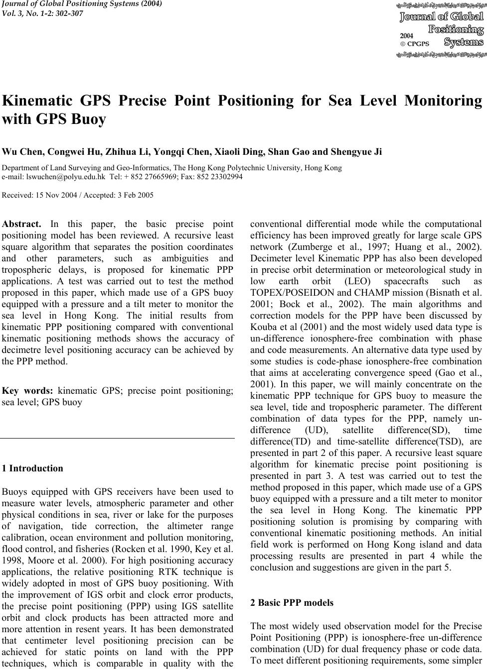Journal of Global Positioning Systems (2004)
Vol. 3, No. 1-2: 302-307
Kinematic GPS Precise Point Positioning for Sea Level Monitoring
with GPS Buoy
Wu Chen, Congwei Hu, Zhihua Li, Yongqi Chen, Xiaoli Ding, Shan Gao and Shengyue Ji
Department of Land Surveying and Geo-Informatic s , The Hong Kong Polytechnic University, H on g K on g
e-mail: lswuchen@poly u.e du .h k T el : + 85 2 27 66 5969; Fax: [phone]
Received: 15 Nov 2004 / Accepted: 3 Feb 2005
Abstract. In this paper, the basic precise point
positioning model has been reviewed. A recursive least
square algorithm that separates the position coordinates
and other parameters, such as ambiguities and
tropospheric delays, is proposed for kinematic PPP
applications. A test was carried out to test the method
proposed in this paper, which made use of a GPS buoy
equipped with a pressure and a tilt meter to monitor the
sea level in Hong Kong. The initial results from
kinematic PPP positioning compared with conventional
kinematic positioning methods shows the accuracy of
decimetre level positioning accuracy can be achieved by
the PPP method.
Key words: kinematic GPS; precise point positioning;
sea level; GPS buoy
1 Introduction
Buoys equipped with GPS receivers have been used to
measure water levels, atmospheric parameter and other
physical conditions in sea, river or lake for the purposes
of navigation, tide correction, the altimeter range
calibration, ocean environment and pollution monitoring,
flood control, and fisheries (Rocken et al. 1990, Key et al.
1998, Moore et al. 2000). For high positioning accuracy
applications, the relative positioning RTK technique is
widely adopted in most of GPS buoy positioning. With
the improvement of IGS orbit and clock error products,
the precise point positioning (PPP) using IGS satellite
orbit and clock products has been attracted more and
more attention in resent years. It has been demonstrated
that centimeter level positioning precision can be
achieved for static points on land with the PPP
techniques, which is comparable in quality with the
conventional differential mode while the computational
efficiency has been improved greatly for large scale GPS
network (Zumberge et al., 1997; Huang et al., 2002).
Decimeter level Kinematic PPP has also been developed
in precise orbit determination or meteorological study in
low earth orbit (LEO) spacecrafts such as
TOPEX/POSEIDON and CHAMP mission (Bisnath et al.
2001; Bock et al., 2002). The main algorithms and
correction models for the PPP have been discussed by
Kouba et al (2001) and the most widely used data type is
un-difference ionosphere-free combination with phase
and code measurements. An alternative data type used by
some studies is code-phase ionosphere-free combination
that aims at accelerating convergence speed (Gao et al.,
2001). In this paper, we will mainly concentrate on the
kinematic PPP technique for GPS buoy to measure the
sea level, tide and tropospheric parameter. The different
combination of data types for the PPP, namely un-
difference (UD), satellite difference(SD), time
difference(TD) and time-satellite difference(TSD), are
presented in part 2 of this paper. A recursive least square
algorithm for kinematic precise point positioning is
presented in part 3. A test was carried out to test the
method proposed in this paper, which made use of a GPS
buoy equipped with a pressure and a tilt meter to monitor
the sea level in Hong Kong. The kinematic PPP
positioning solution is promising by comparing with
conventional kinematic positioning methods. An initial
field work is performed on Hong Kong island and data
processing results are presented in part 4 while the
conclusion and suggestions are given in the part 5.
2 Basic PPP models
The most widely used observation model for the Precise
Point Positioning (PPP) is ionosphere-free un-difference
combination (UD) for dual frequency phase or code data.
To meet different positioning requirements, some simpler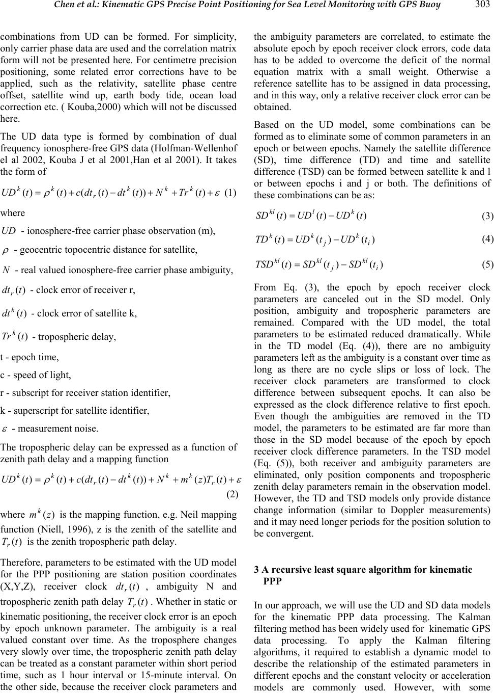

Chen et al.: Kinematic GPS Precise Point Positioning for Sea Level Monitoring with GPS Buoy 303
combinations from UD can be formed. For simplicity,
only carrier phase data are used and the correlation matrix
form will not be presented here. For centimetre precision
positioning, some related error corrections have to be
applied, such as the relativity, satellite phase centre
offset, satellite wind up, earth body tide, ocean load
correction etc. ( Kouba,2000 ) which will not b e discussed
here.
The UD data type is formed by combination of dual
frequency ionosphere-free GPS data (Holfman-Wellenhof
el al 2002, Kouba J et al 2001,Han et al 2001). It takes
the form of
ερ +++−+= )())()(()()( tTrNtdttdtcttUD kkk
r
kk (1)
where
UD - ionosphere-free carrier phase observation (m),
ρ
- geocentric topocentric distance for satellite,
N - real valued ionosphere-free carrier phase ambiguity,
)(tdtr - clock error of receiver r,
)(tdtk - clock error of satellite k,
)(tTrk - tropospheric delay,
t - epoch time,
c - speed of light,
r - subscript for receiver station identifier,
k - superscript for satellite identifier,
ε
- measurement noise.
The tropospheric delay can be expressed as a function of
zenith path delay and a mapping function
ερ +++−+= )()())()(()()( tTzmNtdttdtcttUDr
kkk
r
kk
(2)
where )(zmk is the mapping function, e.g. Neil mapping
function (Niell, 1996), z is the zenith of the satellite and
)(tTr is the zenith tropospheric path delay.
Therefore, parameters to be estimated with the UD model
for the PPP positioning are station position coordinates
(X,Y,Z), receiver clock )(tdtr, ambiguity N and
tropospheric zenith p ath delay )(tTr. Whether in static or
kinematic positioning, the receiver clock error is an epoch
by epoch unknown parameter. The ambiguity is a real
valued constant over time. As the troposphere changes
very slowly over time, the tropospheric zenith path delay
can be treated as a constant parameter within short period
time, such as 1 hour interval or 15-minute interval. On
the other side, because the receiver clock parameters and
the ambiguity parameters are correlated, to estimate the
absolute epoch by epoch receiver clock errors, code data
has to be added to overcome the deficit of the normal
equation matrix with a small weight. Otherwise a
reference satellite has to be assigned in data processing,
and in this way, only a relative receiver clock error can be
obtained.
Based on the UD model, some combinations can be
formed as to eliminate some of common parameters in an
epoch or between epochs. Namely the satellite difference
(SD), time difference (TD) and time and satellite
difference (TSD) can be formed between satellite k and l
or between epochs i and j or both. The definitions of
these combinations can be as:
)()()( tUDtUDtSD klkl −= (3)
)()()( i
k
j
kk tUDtUDtTD−= (4)
)()()( i
kl
j
klkl tSDtSDtTSD −= (5)
From Eq. (3), the epoch by epoch receiver clock
parameters are canceled out in the SD model. Only
position, ambiguity and tropospheric parameters are
remained. Compared with the UD model, the total
parameters to be estimated reduced dramatically. While
in the TD model (Eq. (4)), there are no ambiguity
parameters left as the ambiguity is a constant over time as
long as there are no cycle slips or loss of lock. The
receiver clock parameters are transformed to clock
difference between subsequent epochs. It can also be
expressed as the clock difference relative to first epoch.
Even though the ambiguities are removed in the TD
model, the parameters to be estimated are far more than
those in the SD model because of the epoch by epoch
receiver clock difference parameters. In the TSD model
(Eq. (5)), both receiver and ambiguity parameters are
eliminated, only position components and tropospheric
zenith delay parameters remain in the observation model.
However, the TD and TSD models only provide distance
change information (similar to Doppler measurements)
and it may need longer periods for the position solution to
be convergent.
3 A recursiv e l e a s t s q u a re a lgorith m fo r kinematic
PPP
In our approach, we will use the UD and SD data models
for the kinematic PPP data processing. The Kalman
filtering method has been widely used for kinematic GPS
data processing. To apply the Kalman filtering
algorithms, it required to establish a dynamic model to
describe the relationship of the estimated parameters in
different epochs and the constant velocity or acceleration
models are commonly used. However, with some

304 Journal of Global Positioning Systems
applications, such as GPS buoys, the above models
cannot be used to describe the motion of the GPS
receiver. In this paper a recursive least square method is
proposed to separate the ambiguity and position
parameters. Assuming that there are two kinds of
parameters to be estimated as X and Y, the observation
equation can be written as
PVLBYAX ,+=+ (6)
where X is a vector for coordinate, receiver clock
parameters which need to be estimated at each epoch. Y
is a vector for ambiguity, zenith tropospheric parameter
which does change rapidly between epochs. P is the
weight matrix. The algorithm used in this paper tries to
simplify the observation equation by eliminating
parameter X in the observation equation (Eq. (6)). The
normal equation for Eq. (6) can be written as:
⎥
⎥
⎦
⎤
⎢
⎢
⎣
⎡
=
⎥
⎦
⎤
⎢
⎣
⎡
=
⎥
⎥
⎦
⎤
⎢
⎢
⎣
⎡
PLB
PLA
NN
NN
PBBPAB
PBAPAA
T
T
TT
TT
2221
1211 (7)
with ⎥
⎦
⎤
⎢
⎣
⎡
−IZ
I0，and 1
1121 −
=NNZ (8)
⎥
⎥
⎦
⎤
⎢
⎢
⎣
⎡
=
⎥
⎦
⎤
⎢
⎣
⎡
=
⎥
⎦
⎤
⎢
⎣
⎡
⎥
⎦
⎤
⎢
⎣
⎡
−PLB
PLA
N
NN
NN
NN
IZ
I
T
T
22
1211
2221
1211 0
0
PBAPANBPBBN TTT 1
1122 −
−= (9)
Assuming PAANJ T1
11
−
= (10)
we have
BJIPJIBN TT )()(
22 −−= (11)
with BJIB )( −= (12)
Then we have new normal equation
PLB
Y
B
P
BTT =
This is equivalent to that we have a new observation
equation
PULYB,+= (13)
In Eq. (13) only the parameter Y, such as ambiguity and
tropospheric parameters are included while coordinate
parameter X is eliminated. On the other hand, the
observable L and its weight matrix keep unchanged.
Therefore, in our algorithms, we will estimate the
parameter Y first, together with a simple dynamic model
to describe the ambiguity and tropospheric delays, by
applying a Kalman filter. After parameter Y is
determined, the parameter X (i.e. the station coordinates
and receiver clock errors) can be estimated using the
following equation.
)( 12
1
11 YNPLANX T−= − (14)
4 Data processing results
In this paper, two sets of data are used to demonstrate the
positioning results using the algorithm proposed in the
section 3. The first data set is static GPS data observed in
Hong Kong. The d ata were observ ed on Mar ch 4, 2001 in
Hong Kong GPS active network, totally 24 hours with 5
seconds observation interval. The data is processing in
both state mode (to estimate one solution with all data
available) and the kinematic mode (to estimate position
every epoch). Figure 1 position errors in 3D with the
static mode. It can be seen that it requires about 2 hours
for the coordinate errors to reduce to less than 0.1 m.
With 24 hour data, the coordinate difference compared
with the known coordinate are 0.008m, -0.028m and -
0.001m in north, east and height components. In the
kinematic mode, we solved for the ambiguities and
tropospheric delay parameters first. Then the position
coordinates are solved every epoch in a 5 second interval
using Eq. (14). In data processing, the IGS precise orbit
and 5 min satellite clock error data are used. As in the
kinematic mode 5 second interval data is used, we use a
linear interpolation of 5 minute satellite clock error to get
the satellite clock errors at the epoch. Figure 2(a) shows
the position errors with 5 second interval. The position
RMS errors with 5 second interval d a ta are 0.0 37 m, 0.043
and 0.104m in North, East and Height component
respectively. To assess the errors caused by the
interpolation of satellite clock errors, we process the data
again with 5 minute interval, with the epoch we have
exact satellite clock errors as IGS provided. The
positioning errors are shown in Figure 2(b). Comparing
Figures 2(a) and (2(b), it can be seen that position errors
with the epochs that have the exact IGS clock error
(Figure 2(b)) are much less the solution with the
interpolated satellite clock error (Figure 2(a)). The
position RMS errors with the solution that is without
using the clock interpolation are 0.021m,0.030m and
0.055m in North, East and Height component
respectively. This clearly shows that the satellite clock
accuracy plays an important role on the PPP method.
To test the overall performance of the kinematic PPP
method in a kinematic environment, we use GPS buoy
data with 1s data interval, from 22 to 24 October 2004, at
Repulse Bay, Hong Kong island. Two Leica SR530 dual
frequency GPS receivers were used, one is set on shore as
a fixed station for differential positioning test and another
receiver is installed on a buoy in the sea. (Figure 3).
Firstly we estimate the position of GPS buoy with the
relative position mode. As the reference station is very
close to the GPS buoy (a few hundred metres), most GPS
measurement errors can be cancelled out by the relative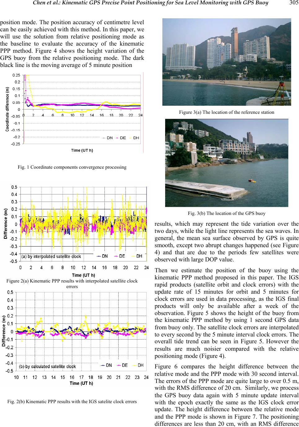

Chen et al.: Kinematic GPS Precise Point Positioning for Sea Level Monitoring with GPS Buoy 305
position mode. The position accuracy of centimetre level
can be easily achieved with this method. In this paper, we
will use the solution from relative positioning mode as
the baseline to evaluate the accuracy of the kinematic
PPP method. Figure 4 shows the height variation of the
GPS buoy from the relative positioning mode. The dark
black line is the moving average of 5 minute position
Fig. 1 Coordinate components convergence processi n g
Figure 2(a) Kinematic PPP results with interpolated satellite clock
errors
Fig. 2(b) Kinematic PPP results with the IGS satelite clock errors
Figure 3(a) The location of the reference station
Fig. 3(b) The location of the GPS buoy
results, which may represent the tide variation over the
two days, while the light line represents the sea waves. In
general, the mean sea surface observed by GPS is quite
smooth, except two abrupt changes happened (see Figure
4) and that are due to the periods few satellites were
observed with large DOP value.
Then we estimate the position of the buoy using the
kinematic PPP method proposed in this paper. The IGS
rapid products (satellite orbit and clock errors) with the
update rate of 15 minutes for orbit and 5 minutes for
clock errors are used in data processing, as the IGS final
products will only be available after a week of the
observation. Figure 5 shows the height of the buoy from
the kinematic PPP method by using 1 second GPS data
from buoy only. The satellite clock errors are interpolated
to every second by the 5 minute interval clock errors. The
overall tide trend can be seen in Figure 5. However the
results are much noisier compared with the relative
positioning mode (Figure 4).
Figure 6 compares the height difference between the
relative mode and the PPP mode with 30 second interval.
The errors of the PPP mode are quite large to over 0.5 m,
with the RMS difference of 20 cm. Similarly, we process
the GPS buoy data again with 5 minute update interval
with the epoch exactly the same as the IGS clock error
update. The height difference between the relative mode
and the PPP mode is shown in Figure 7. The positioning
differences are less than 20 cm, with an RMS difference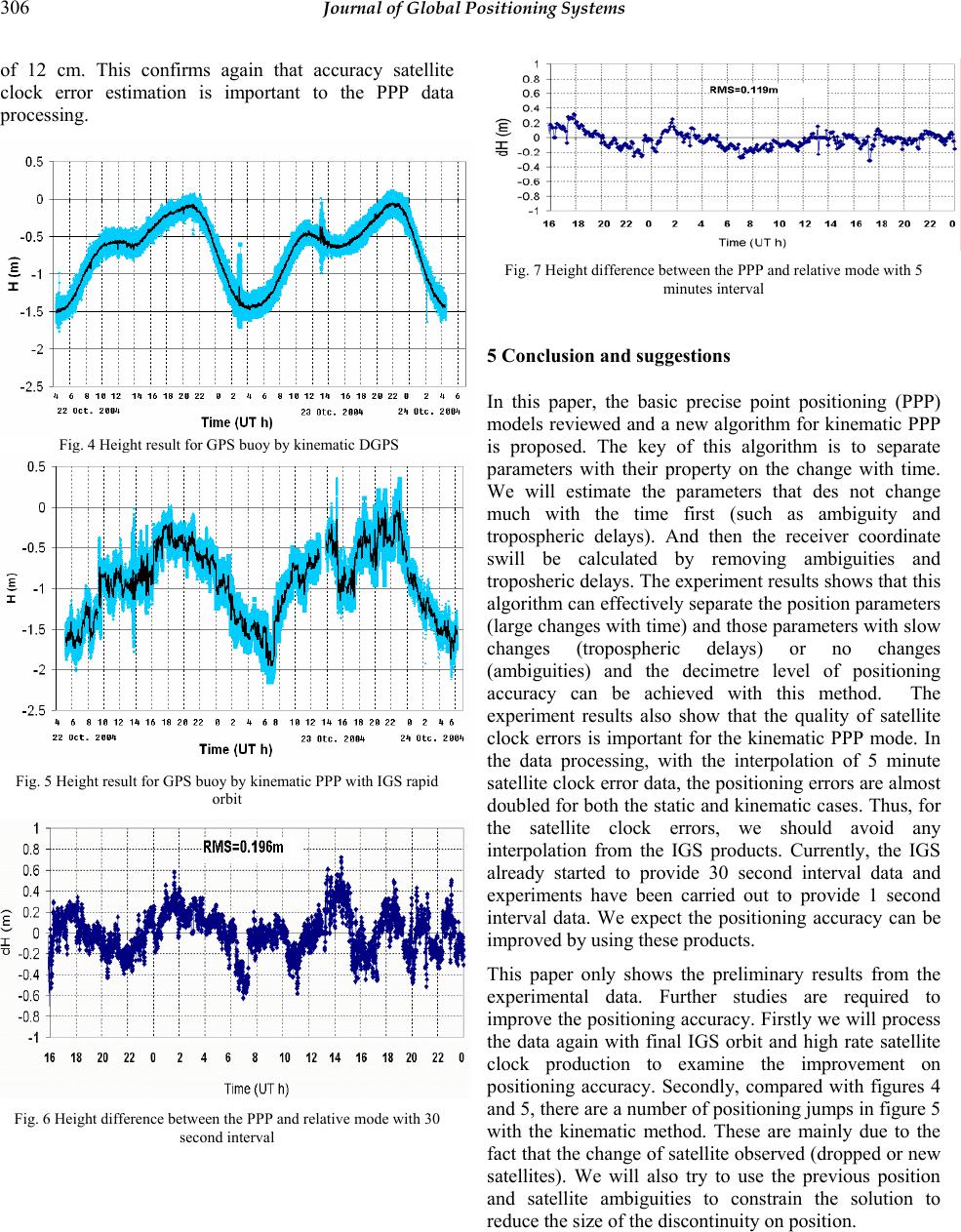

306 Journal of Global Positioning Systems
of 12 cm. This confirms again that accuracy satellite
clock error estimation is important to the PPP data
processing.
Fig. 4 Height result for GPS buoy by kinematic DGPS
Fig. 5 Height result for GPS buoy by kinematic PPP with IGS rapid
orbit
Fig. 6 Height difference between the PPP and relative mode with 30
second interval
Fig. 7 Height difference between th e PPP and relative mode with 5
minutes interval
5 Conclusion a nd suggestio ns
In this paper, the basic precise point positioning (PPP)
models reviewed and a new algorithm for kinematic PPP
is proposed. The key of this algorithm is to separate
parameters with their property on the change with time.
We will estimate the parameters that des not change
much with the time first (such as ambiguity and
tropospheric delays). And then the receiver coordinate
swill be calculated by removing ambiguities and
troposheric delays. The experiment results shows that this
algorithm can effectively separate the position parameters
(large changes with time) and those parameters with slow
changes (tropospheric delays) or no changes
(ambiguities) and the decimetre level of positioning
accuracy can be achieved with this method. The
experiment results also show that the quality of satellite
clock errors is important for the kinematic PPP mode. In
the data processing, with the interpolation of 5 minute
satellite clock error data, the positioning errors are almost
doubled for both the static and kinematic cases. Thus, for
the satellite clock errors, we should avoid any
interpolation from the IGS products. Currently, the IGS
already started to provide 30 second interval data and
experiments have been carried out to provide 1 second
interval data. We expect the positioning accuracy can be
improved by using these products.
This paper only shows the preliminary results from the
experimental data. Further studies are required to
improve the positioning accuracy. Firstly we will process
the data again with final IGS orbit and high rate satellite
clock production to examine the improvement on
positioning accuracy. Secondly, compared with figures 4
and 5, there are a number of positioning jumps in figure 5
with the kinematic method. These are mainly due to the
fact that the change of satellite observed (dropped or new
satellites). We will also try to use the previous position
and satellite ambiguities to constrain the solution to
reduce the size of the discontinuity on position.

Chen et al.: Kinematic GPS Precise Point Positioning for Sea Level Monitoring with GPS Buoy 307
ACKNOWLEDGEMENTS
This study is under the support by the Hong Kong RGC projects:
PolyU 5075/01E and PolyU 5062/02E.
References
Han SC, Kwon JH, Jekeli C (2001): Accurate Absolute GPS
Positioning through Satellite Clock Error Estimation,
Journal of Geodesy, 77: 33 - 43.
Héroux P.; Kouba J (2001): GPS Precise Point Positioning
Using IGS Orbit Products. Physics and Chemistry of the
Earth (A), Vol. 26 No. 6 – 8: 573 – 578.
Hofmann-Wellenhof B.; Lichtenegger H.; Collins J. (2003):
GPS Theory and Practice (5th Ed.). Springer, Wien New
York.
Moore T.; Zhang K.; Close G.; Moore R. (2000): Real-Time
River Level Monitoring Using GPS Heighting. GPS
Solution, Vol. 4, Number 2: 63 - 67.
Key K.W.; Parke M.E.; Norn G.H. (1998): Mapping the Sea
Surface Using a GPS Buoy. Marine Geodesy, 21: 67 –
79.
Niell; A. E. (1996): Global Mapping Functions for the
Atmosphere Delay at Radio Wavelengths. Journal of
Geophysical Research, 101(B2): 3227 - 3246.
Rocken C.; Kelecy T.M.; Norn G.H.; Young L.E.; Purcell G.H.;
Jr.; Wolf S.K. (1990): Measuring Precise Sea Level From
a Buoy Using the Global Positioning System. Geophysical
Research Letters, 17: 2145 – 2148.
Zumberge JF; Watkins MM; Web FH (1998): Characters and
Applications of Precise GPS Clock Solutions of Every 30
Seconds. Journal of the Institute of Navigation, 44(4): 449
– 456.
Zumberge JF; Heflin MB; Jefferson DC; Watkins MM; Webb
FH (1997): Precise Point Processing for the Efficient and
Robust Analysis of GPS Data from Large Networks.
Journal of Geophysical Research, 102 (B3): 5005 - 5017.