Paper Menu >>
Journal Menu >>
 Int. J. Communications, Network and System Sciences, 2010, 3, 805-810 doi:10.4236/ijcns.2010.310108 Published Online October 2010 (http://www.SciRP.org/journal/ijcns) Copyright © 2010 SciRes. IJCNS Performance Improvement of Wi reless Communications Using Frequency Hopping Spread Spectrum Naser Hossein Motlagh Department of Information Techn ol o gy, V aas a Uni versit y o f Appli e d Scie n ces, Vaa sa , Fi nl a nd E-mail: nah@puv.fi Received June 18, 201 0; revised August 1, 2010; accepted Septe mber 6, 2010 Abstract To improve the performance of short-range wireless communications, channel quality must be improved by avoiding interference and multi-path fading. Frequency hopping spread spectrum (FHSS) is a transmission technique where the carrier hops from frequency to frequency. For frequency hopping a mechanism must be designed so that the data can be transmitted in a clear channel and avoid congested channels. Adaptive fre- quency hopping is a system which is used to improve immunity toward frequency interference by avoiding using congested frequency channels in hopping sequence. In this paper mathematical modelling is used to simulate and analyze the performance improvement by using FHSS with popular modulation schemes, and also the hopping channel situations are investigated. Keywords: Frequency Hopping Spread Spectrum, Adaptive Frequency Hopping, Performance Evaluation 1. Introduction In this paper the focus is to improve wireless communi- cation performance by adaptive frequency hopping which is implemented by selecting sets of communication chan- nels and adaptively hopping sender’s and receiver’s fre- quency channels and determining the channel numbers with less interference. Also the work investigates whe ther the selected channels are congested or clear then a list of good channels can be generated and in practice to use detected frequency channels as hopping sequence to im- prove the performance of communication and finally the quality of service. The Fourier transform mathematical modules are used to convert signals from time domain to frequency do- main and vice versa. The mathematical modules are ap- plied to represent the frequency and simulate them in MATLAB and as result the simulated spectrums are an- alysed. Then a simple two-state Gilbert-Elliot Channel Model [1,2] in which a two-state Markov chain with states named “Good” and “Bad” is used to check if the channels are congested or clear in case of interference. Finally, a solution to improve the performance of wire- less communications by choosing and using “Good” channels as the next frequency hopping sequence chan- nel is proposed. 2. Review of Related Theories 2.1. Spread Spectrum Spread spectrum is a digital modulation technology and a technique based on principle of spreading a signal among many frequencies to prevent interference and signal in- terception [3]. As the name shows it is a technique to spread the transmitted spectrum over a wide range of frequencies. It started to be employed by military appli- cations because of its Low Probability of Intercept or demodulation, interference and anti-jamming from en- emy side. The idea of spreading spectrum is to spread a signal over a large frequency band to use greater band- width than the data bandwidth while the power remains the same. And as far as the spread signal looks like the noise signal in the same frequency band it is difficult to recognize the signal which this feature of spreading pro- vides security to the transmission. Compared to a nar- rowband signal, spread spectrum spreads the signal power over a wideband and the overall SNR is improved because only a small part of spread spectrum signal is affected by interference. In sender and receiver sides of a communication system one spreading generator is lo- cated based on the spreading technique they synchronize the received modulated spectrum. Shannon capacity Eq- 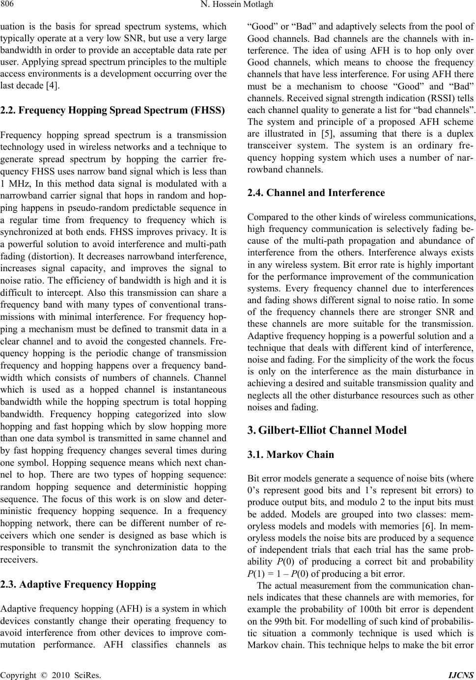 N. Hossein Motlagh Copyright © 2010 SciRes. IJCNS 806 uation is the basis for spread spectrum systems, which typically operate at a very low SNR, but use a very large bandwidth in order to provide an acceptable data rate per user. Applying spread spectrum principles to th e multiple access environments is a development occurring over the last decade [4]. 2.2. Frequency Hopping Spread Spectrum (FHSS) Frequency hopping spread spectrum is a transmission technology used in wireless networks and a technique to generate spread spectrum by hopping the carrier fre- quency FHSS uses narrow band signal which is less than 1 MHz, In this method data signal is modulated with a narrowband carrier signal that hops in random and hop- ping happens in pseudo-random predictable sequence in a regular time from frequency to frequency which is synchronized at both ends. FHSS improves privacy. It is a powerful solution to avoid interference and multi-path fading (distortion). It decreases narrowband interference, increases signal capacity, and improves the signal to noise ratio. The efficiency of bandwidth is high and it is difficult to intercept. Also this transmission can share a frequency band with many types of conventional trans- missions with minimal interference. For frequency hop- ping a mechanism must be defined to transmit data in a clear channel and to avoid the congested channels. Fre- quency hopping is the periodic change of transmission frequency and hopping happens over a frequency band- width which consists of numbers of channels. Channel which is used as a hopped channel is instantaneous bandwidth while the hopping spectrum is total hopping bandwidth. Frequency hopping categorized into slow hopping and fast hopping which by slow hopping more than one data symbol is tran smitted in same channel and by fast hopping frequency changes several times during one symbol. Hopping sequence means which next chan- nel to hop. There are two types of hopping sequence: random hopping sequence and deterministic hopping sequence. The focus of this work is on slow and deter- ministic frequency hopping sequence. In a frequency hopping network, there can be different number of re- ceivers which one sender is designed as base which is responsible to transmit the synchronization data to the receivers. 2.3. Adaptive Frequency Hopping Adaptiv e frequency hopping (AFH) is a system in which devices constantly change their operating frequency to avoid interference from other devices to improve com- mutation performance. AFH classifies channels as “Good” or “Bad” and adaptively selects from the pool of Good channels. Bad channels are the channels with in- terference. The idea of using AFH is to hop only over Good channels, which means to choose the frequency channels that have less interferen ce. For using AFH th ere must be a mechanism to choose “Good” and “Bad” channels. Received signal strength indication (RSSI) tells each channel quality to generate a list for “bad channels”. The system and principle of a proposed AFH scheme are illustrated in [5], assuming that there is a duplex transceiver system. The system is an ordinary fre- quency hopping system which uses a number of nar- rowband channels. 2.4. Channel and Interference Compared to the other kinds of wireless communications, high frequency communication is selectively fading be- cause of the multi-path propagation and abundance of interference from the others. Interference always exists in any wireless system. Bit error rate is highly important for the performance improvement of the communication systems. Every frequency channel due to interferences and fading shows different signal to noise ratio. In some of the frequency channels there are stronger SNR and these channels are more suitable for the transmission. Adaptive frequen cy hopping is a powerful so lution and a technique that deals with different kind of interference, noise and fading. For the simplicity of the work the focus is only on the interference as the main disturbance in achieving a desired and suitable tran smission quality and neglects all the other disturbance resources such as other noises and fading. 3. Gilbert-Elliot Channel Model 3.1. Markov Chain Bit error models generate a sequence of noise bits (where 0’s represent good bits and 1’s represent bit errors) to produce output bits, and modulo 2 to the input bits must be added. Models are grouped into two classes: mem- oryless models and models with memories [6]. In mem- oryless models the noise bits are produced by a sequence of independent trials that each trial has the same prob- ability P(0) of producing a correct bit and probability P(1) = 1 – P(0) of producing a bit error. The actual measurement from the communication chan- nels indicates that these channels are with memories, for example the probability of 100th bit error is dependent on the 99th bit. For modellin g of such kind of probabilis- tic situation a commonly technique is used which is Markov chain. This technique helps to make the bit error  N. Hossein Motlagh Copyright © 2010 SciRes. IJCNS 807 probability depend on the states. The use of Markov chain in bit error models has been introduced by Gil- bert-Elliot for the first time. Gilbert-Elliot channel model based on Markov chain has two states G (Good) and B (Bad). In state G, transmission is error-free and in sate B the link has probability h of transmitting a bit correctly. Figure 1 shows a transition diagram and bit error prob- abilities for Markov chain. The model has three inde- pendent parameters (p, P and h) to describe the error performance of wireless links. The situation of small p is where transition jumps from B to G and the capital P is where transition jumps from G to B. Also the states B and G tend to persist and the model simulates bursts of errors. The parameters p, P and h are not directly observable and therefore must be determined from statistic meas- urements of the error process. It’s also important to note that runs of G alternates with runs of B. The run length has geometric distributions, with mean 1/P for the G-runs and 1/p for the B-runs. 3.2. Geometric Distribution The run lengths of Good and Bad states can be expressed by geometric distribution in which for the Good runs, mean value of 1/P and for the Bad runs, the mean value of 1/p is used. The time fraction in both of Good and Bad states based on persistence in each state can be calculated, for example the fraction of time spent in B state is: () P PB Pp (1) The sequence of states cannot be reconstructed from the sequence of bits in the error process, because both of 0’s and 1’s (the Good bits and Bad bits) are produced in the B state and since bit errors happen only in state B with probability of 1-h then the probability of error is: (1)(1,)()(1|)(1) P PPBPBPBh Pp (2) Figure 1. Transition diagram and bit error probabilities model. The bits of the error process (runs of 0’s and 1’s) and the distribution of run lengths of 0’s (error gaps) and 1’s (error bursts) are observable to determine model pa- rameters. 3.3. Parameter Estimation The determination of the three parameters p, P, and h from measurements of the error process requires that pa- rameters be expressed as functions of three other parame- ters that are directly observable. For Markov chain pa- rameter estimation the functions have been proved for- merly [6]: 1 1(1) EB qh (3) (1) (1) (1 )(1)[1(1 )] EG hQ q hQqh (4) 2(1 ) 1(1) EB qh qh (5) 22 3 (1)() (1)[] [1(1 )]()(1) E GEG hqJp QJJJL qhJL J (6) In the Equations E B is the mean error bust length and E G is the mean error gap length, 2 E B is the variance of the error burst distribution and 2 E B is the variance of error gap distribution. J and L are defined as: 2 2()4() J Qhq QhqhpQ (7) 2 2()4()LQhq QhqhpQ (8) 4. Matlab Modelling 4.1. Gilbert-Elliot Modelling Gilbert-Elliot channel model is used for modelling a tel- ecommunication channel. For obtaining the parameters of this model, first a sequence of data bit is given to the transmitter and then from the receiver side the transmit- ted data is received as output data. With the input se- quence and output sequence, bit error sequence can be calculated easily. By having this bit error sequence and the method of parameter estimation in [6] the model pa- rameters can be calculated. For this reason channel simulation is done with Simu- link. To obtain the bit sequence of input and output, two variables with names “in” and “out” are used. With XORing the input and output bit sequences the bit error sequence is calculated. By setting bit error sequence at argument of function marcov, Markov parameters can be achieved from the output of function marcov. In function 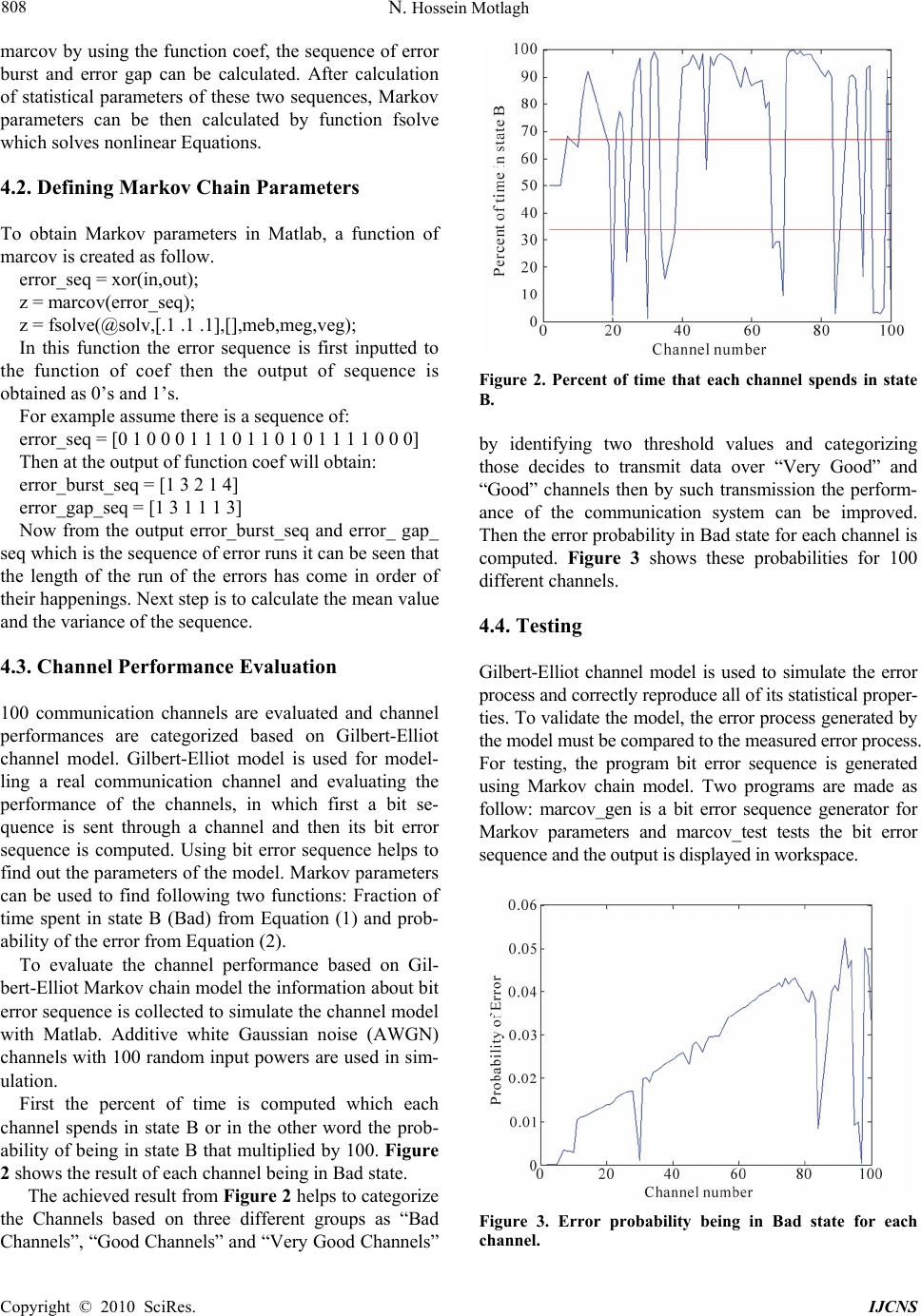 N. Hossein Motlagh Copyright © 2010 SciRes. IJCNS 808 marcov by using the function coef, the sequence of error burst and error gap can be calculated. After calculation of statistical parameters of these two sequences, Markov parameters can be then calculated by function fsolve which solves no nlinear Equations. 4.2. Defining Markov Chain Parameters To obtain Markov parameters in Matlab, a function of marcov is created as follow. error_seq = xor(in,out); z = marcov(error_seq); z = fsolve(@solv,[.1 .1 .1],[],meb,meg,veg); In this function the error sequence is first inputted to the function of coef then the output of sequence is obtained as 0’s and 1’s. For example assume there is a sequence of: error_seq = [0 1 0 0 0 1 1 1 0 1 1 0 1 0 1 1 1 1 0 0 0] Then at the outpu t of function coef will obtain: error_burst_seq = [1 3 2 1 4] error_gap_seq = [1 3 1 1 1 3] Now from the output error_burst_seq and error_ gap_ seq which is the sequence of error runs it can be seen that the length of the run of the errors has come in order of their happenings. Next step is to calculate the mean value and the variance of the sequence. 4.3. Channel Performance Evaluation 100 communication channels are evaluated and channel performances are categorized based on Gilbert-Elliot channel model. Gilbert-Elliot model is used for model- ling a real communication channel and evaluating the performance of the channels, in which first a bit se- quence is sent through a channel and then its bit error sequence is computed. Using bit error sequence helps to find out the parameters of the model. Markov parameters can be used to find following two functions: Fraction of time spent in state B (Bad) from Equation (1) and prob- ability of the error from Equation (2). To evaluate the channel performance based on Gil- bert-Elliot Markov ch ain model the information abou t bit error sequence is collected to simulate the channel model with Matlab. Additive white Gaussian noise (AWGN) channels with 100 random input powers are used in sim- ulation. First the percent of time is computed which each channel spends in state B or in the other word the prob- ability of being in state B that multiplied by 100. Figure 2 shows the result of each channel being in Bad state. The achieved result from Figure 2 helps to categorize the Channels based on three different groups as “Bad Channels”, “Good Channels” and “Very Good Channels” Figure 2. Percent of time that each channel spends in state B. by identifying two threshold values and categorizing those decides to transmit data over “Very Good” and “Good” channels then by such transmission the perform- ance of the communication system can be improved. Then the error probab ility in Bad state for each channel is computed. Figure 3 shows these probabilities for 100 different channels. 4.4. Testing Gilbert-Elliot channel model is used to simulate the error process and correctly reproduce all of its statistical proper- ties. To validate the model, the error process generated by the model must be compared to the measured error process. For testing, the program bit error sequence is generated using Markov chain model. Two programs are made as follow: marcov_gen is a bit error sequence generator for Markov parameters and marcov_test tests the bit error sequence and the output is displayed in workspace. Figure 3. Error probability being in Bad state for each channel.  N. Hossein Motlagh Copyright © 2010 SciRes. IJCNS 809 The objective of the parameter estimation is to choose values of the model parameters that generate error burst and error gap distributions that reassembles the corresponding measured distributions as close as possible. Therefore for testing the mean and variance of error burst and error gap of regenerated error sequence are calculated and compared by statistical parameters of channel bit error sequence, where the result is shown in Table 1. A: Statistical parameters channel error sequence. B: Statistical parameters of regenerated error sequence. For testing, first Markov model parameters of a chan- nel error sequence are computed, then a sequence of the model is generated and statistical parameters are com- puted. The statistical parameters must be as equal as channel error sequence. It is important to mention that first state of the Markov model in function marcov_gen chooses the probability 0.5, so sometimes two different answers can be seen and that the nearest one to the error sequence statistic is the correct one. 5. Evaluation of Frequency Hopping To design the frequency hopping (FH) model, MATLA B Simulink has been used. The spreader at transmitter sec- tion is an M-FSK modulation but the input of the modu- lator is hopping index. This section consists of a PN Se- quence Generator, an Assemble Packets block and a Go- to block as shown in Figure 4. The design of frequency hopping spreader is shown in Figure 5. The spreader part consists of M-FSK modula- tor base (with M equal to 64), a From block (Hop index that is created in previous step), a To Frame block and a Multiplication block. The block parameter of FSK modu- lator is 64 in M-FSK number and it means that there are 64 hopping sections. These sub-bands are selected by the hop indexes. The design of frequency hopping despreader, is the same as spreader section but the output of M-FSK modu- lator block is compl ex conjug ated as shown Figure 6. This frequency hopping model is used for evaluation of three different modulations: QAM, QPSK, GFSK, and compares the performance with the situation without frequency hopping. Performance evaluation is based on BER values under two situations (with and without FH) versus normalized signal-to-noise ratio (SNR) meas- ured by Eb/N0 values of the channel, as shown in Fig- ures 7-9. From Figure 7 it can be seen that applying FH with QAM modulation does not lead to a sensible improve- ment in performance or significant reduction of BER. From Figure 8 it can be seen that applying FH with QPSK modulation gives a good result and reduces significantly BER compared to without FH at same level Table 1. Statistical parameters of channel error and regen- erated error se quence. error burst mean error gap mean error gap variance 1.0568 18.1134 319.4516 A SNR = 3dB Input power = 11.0492 18.4713 319.3184 B 1.1456 7.7868 48.9981 A SNR = 3dB Input power = 21.1500 8.0421 55.0026 B 1.2201 5.6570 25.5754 A SNR = 3dB Input power = 31.2271 5.5166 24.5044 B Figure 4. Model of fre quency hopping in Simulink. Figure 5. Design of frequenc y hopping spr e ader. Figure 6. Design of frequency hopping despreader. of SNR. From Figure 9 it can be seen that applying FH with GFSK modulation reduces dramatically BER com- pared to without FH at same level of SNR and lead to a much higher performance.  N. Hossein Motlagh Copyright © 2010 SciRes. IJCNS 810 Figure 7. QAM modulation. Figure 8. QPSK modulation. Figure 9. GFSK modulation. In overall, based on the evaluation results it can be concluded that applying the designed FH schemes with certain modulations can improve their communication performances, especially at weak SNR levels as most cases of short range wireless communications have. 6. Conclusions As a result it can be concluded that adaptive frequency hopping is a powerful technique to deal with interference and Gilbert-Elliot channel model is a good technique to analyze the situations of channels by categorizing the channel conditions based on their performance as Good or Bad, and then apply adaptive frequency hopping which hops frequencies adaptively by analyzing the state of the channel in case of environmental problems such as interferences and noises to improve the communication performance. Frequency hopping spread spectrum is modelled with MATLAB and three different modula- tions i.e. QAM, QPSK and GFSK are studied to investi- gate which of these modulations are good to apply with FHSS model. The simulation results show that applying FHSS with QAM modulation dose not lead to a remark- able reduction of BER, but with QPSK modulation gives a good result and reduces BER at lower SNR, while in GFSK modulation shows a significant reduction of BER and lead to a high performance. 7. Acknowledgement The author gratefully acknowledges Dr Yang Liu for his valuable support and guidance in this research work. 8. References [1] E. N. Gilbert, “Capacity of Burst-Noise Channels,” Bell System Technical Journal, Vol. 39, 1960, pp. 1253-1265. [2] E. O. Elliott, “Estimates of Error Rates for Codes on Burst-Noise Channels,” Bell System Technical Journal, Vol. 42, 1963, pp. 1977-1997. [3] R. E. Ziemer, R. L. Peterson and D. E. Borth, “Introduc- tion to Spread Spectrum Communications,” Prentice Hall, Englewood Cliffs, New Jersey, 1995. [4] R. J. Bates and D. W. Gregory, “Voice & Data Commu- nications Handbook,” McGraw-Hill Osborne Media, Berke- le y , C A , 2001. [5] J. Zander and G. Malmgren, “Adaptive Frequency Hop- ping in HF Communications,” IEE Proceedings Commu- nications, Vol. 142, No. 2, 1995, pp. 99-105. [6] J. J. Lemmon, “Wireless Link Statistical Bit Error Model,” Institute for Telecommun ica ti on Sci enc es , 2002. |