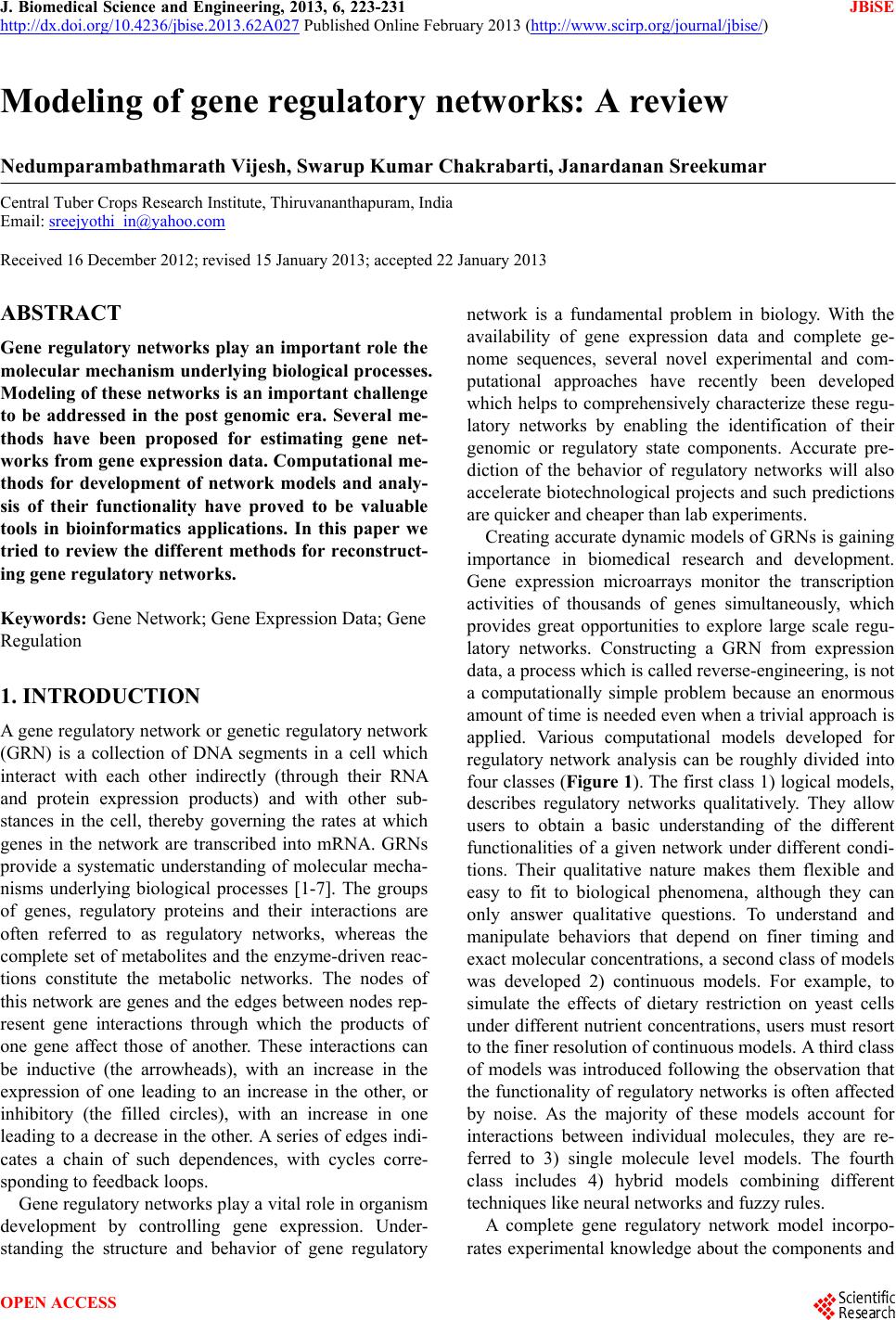
 J. Biomedical Science and Engineering, 2013, 6, 223-231 JBiSE http://dx.doi.org/10.4236/jbise.2013.62A027 Published Online February 2013 (http://www.scirp.org/journal/jbise/) Modeling of gene regulatory networks: A review Nedumparambathmarath Vijesh, Swarup Kumar Chakrabarti, Janardanan Sreekumar Central Tuber Crops Research Institute, Thiruvananthapuram, India Email: sreejyothi_in@yahoo.com Received 16 December 2012; revised 15 January 2013; accepted 22 January 2013 ABSTRACT Gene regulatory networks play an important role the molecular mechanism underlying biological processes. Modeling of these networks is an important challenge to be addressed in the post genomic era. Several me- thods have been proposed for estimating gene net- works from gene expression data. Computational me- thods for development of network models and analy- sis of their functionality have proved to be valuable tools in bioinformatics applications. In this paper we tried to review the different methods for reconstruct- ing gene regulatory networks. Keywords: Gene Network; Gene Expression Data; Gene Regulation 1. INTRODUCTION A gene regulatory network or genetic regulatory network (GRN) is a collection of DNA segments in a cell which interact with each other indirectly (through their RNA and protein expression products) and with other sub- stances in the cell, thereby governing the rates at which genes in the network are transcribed into mRNA. GRNs provide a systematic understanding of molecular mecha- nisms underlying biological processes [1-7]. The groups of genes, regulatory proteins and their interactions are often referred to as regulatory networks, whereas the complete set of metabolites and the enzyme-driven reac- tions constitute the metabolic networks. The nodes of this network are genes and the edges between nodes rep- resent gene interactions through which the products of one gene affect those of another. These interactions can be inductive (the arrowheads), with an increase in the expression of one leading to an increase in the other, or inhibitory (the filled circles), with an increase in one leading to a decrease in the other. A series of edges indi- cates a chain of such dependences, with cycles corre- sponding to feedback loops. Gene regulatory networks play a vital role in organism development by controlling gene expression. Under- standing the structure and behavior of gene regulatory network is a fundamental problem in biology. With the availability of gene expression data and complete ge- nome sequences, several novel experimental and com- putational approaches have recently been developed which helps to comprehensively characterize these regu- latory networks by enabling the identification of their genomic or regulatory state components. Accurate pre- diction of the behavior of regulatory networks will also accelerate biotechnological projects and such predictions are quicker and cheaper than lab experiments. Creating accurate dynamic models of GRNs is gaining importance in biomedical research and development. Gene expression microarrays monitor the transcription activities of thousands of genes simultaneously, which provides great opportunities to explore large scale regu- latory networks. Constructing a GRN from expression data, a process which is called reverse-engineering, is not a computationally simple problem because an enormous amount of time is needed even when a trivial approach is applied. Various computational models developed for regulatory network analysis can be roughly divided into four classes (Figure 1). The first class 1) logical models, describes regulatory networks qualitatively. They allow users to obtain a basic understanding of the different functionalities of a given network under different condi- tions. Their qualitative nature makes them flexible and easy to fit to biological phenomena, although they can only answer qualitative questions. To understand and manipulate behaviors that depend on finer timing and exact molecular concentrations, a second class of models was developed 2) continuous models. For example, to simulate the effects of dietary restriction on yeast cells under different nutrient concentrations, users must resort to the finer resolution of continuous models. A third class of models was introduced following the observation that the functionality of regulatory networks is often affected by noise. As the majority of these models account for interactions between individual molecules, they are re- ferred to 3) single molecule level models. The fourth class includes 4) hybrid models combining different techniques like neural networks and fuzzy rules. A complete gene regulatory network model incorpo- rates experimental knowledge about the components and OPEN ACCESS 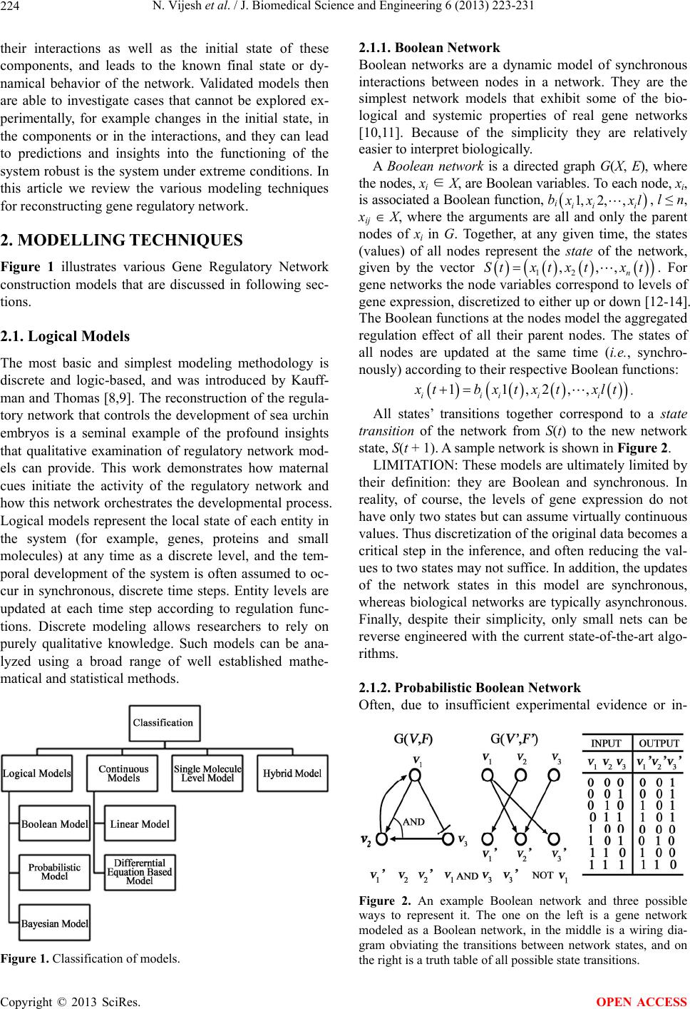 N. Vijesh et al. / J. Biomedical Science and Engineering 6 (2013) 223-231 224 their interactions as well as the initial state of these components, and leads to the known final state or dy- namical behavior of the network. Validated models then are able to investigate cases that cannot be explored ex- perimentally, for example changes in the initial state, in the components or in the interactions, and they can lead to predictions and insights into the functioning of the system robust is the system under extreme conditions. In this article we review the various modeling techniques for reconstructing gene regulatory network. 2. MODELLING TECHNIQUES Figure 1 illustrates various Gene Regulatory Network construction models that are discussed in following sec- tions. 2.1. Logical Models The most basic and simplest modeling methodology is discrete and logic-based, and was introduced by Kauff- man and Thomas [8,9]. The reconstruction of the regula- tory network that controls the development of sea urchin embryos is a seminal example of the profound insights that qualitative examination of regulatory network mod- els can provide. This work demonstrates how maternal cues initiate the activity of the regulatory network and how this network orchestrates the developmental process. Logical models represent the local state of each entity in the system (for example, genes, proteins and small molecules) at any time as a discrete level, and the tem- poral development of the system is often assumed to oc- cur in synchronous, discrete time steps. Entity levels are updated at each time step according to regulation func- tions. Discrete modeling allows researchers to rely on purely qualitative knowledge. Such models can be ana- lyzed using a broad range of well established mathe- matical and statistical methods. Figure 1. Classification of models. 2.1.1. Boolean Network Boolean networks are a dynamic model of synchronous interactions between nodes in a network. They are the simplest network models that exhibit some of the bio- logical and systemic properties of real gene networks [10,11]. Because of the simplicity they are relatively easier to interpret biologically. A Boolean network is a directed graph G(X, E), where the nodes, xi ∈ X, are Boolean variables. To each node, xi, is associated a Boolean function, bi 1, 2,, ii i xxl , l ≤ n, xij X, where the arguments are all and only the parent nodes of xi in G. Together, at any given time, the states (values) of all nodes represent the state of the network, given by the vector 12 ,,, n tx tx tSt x. For gene networks the node variables correspond to levels of gene expression, discretized to either up or down [12-14]. The Boolean functions at the nodes model the aggregated regulation effect of all their parent nodes. The states of all nodes are updated at the same time (i.e., synchro- nously) according to their respective Boolean functions: 11,2,, iiii i tbxtxtxlt . All states’ transitions together correspond to a state transition of the network from S(t) to the new network state, S(t + 1). A sample network is shown in Figure 2. LIMITATION: These models are ultimately limited by their definition: they are Boolean and synchronous. In reality, of course, the levels of gene expression do not have only two states but can assume virtually continuous values. Thus discretization of the original data becomes a critical step in the inference, and often reducing the val- ues to two states may not suffice. In addition, the updates of the network states in this model are synchronous, whereas biological networks are typically asynchronous. Finally, despite their simplicity, only small nets can be reverse engineered with the current state-of-the-art algo- rithms. 2.1.2. Probabilistic Boolean Network Often, due to insufficient experimental evidence or in- Figure 2. An example Boolean network and three possible ways to represent it. The one on the left is a gene network modeled as a Boolean network, in the middle is a wiring dia- gram obviating the transitions between network states, and on the right is a truth table of all possible state transitions. Copyright © 2013 SciRes. OPEN ACCESS 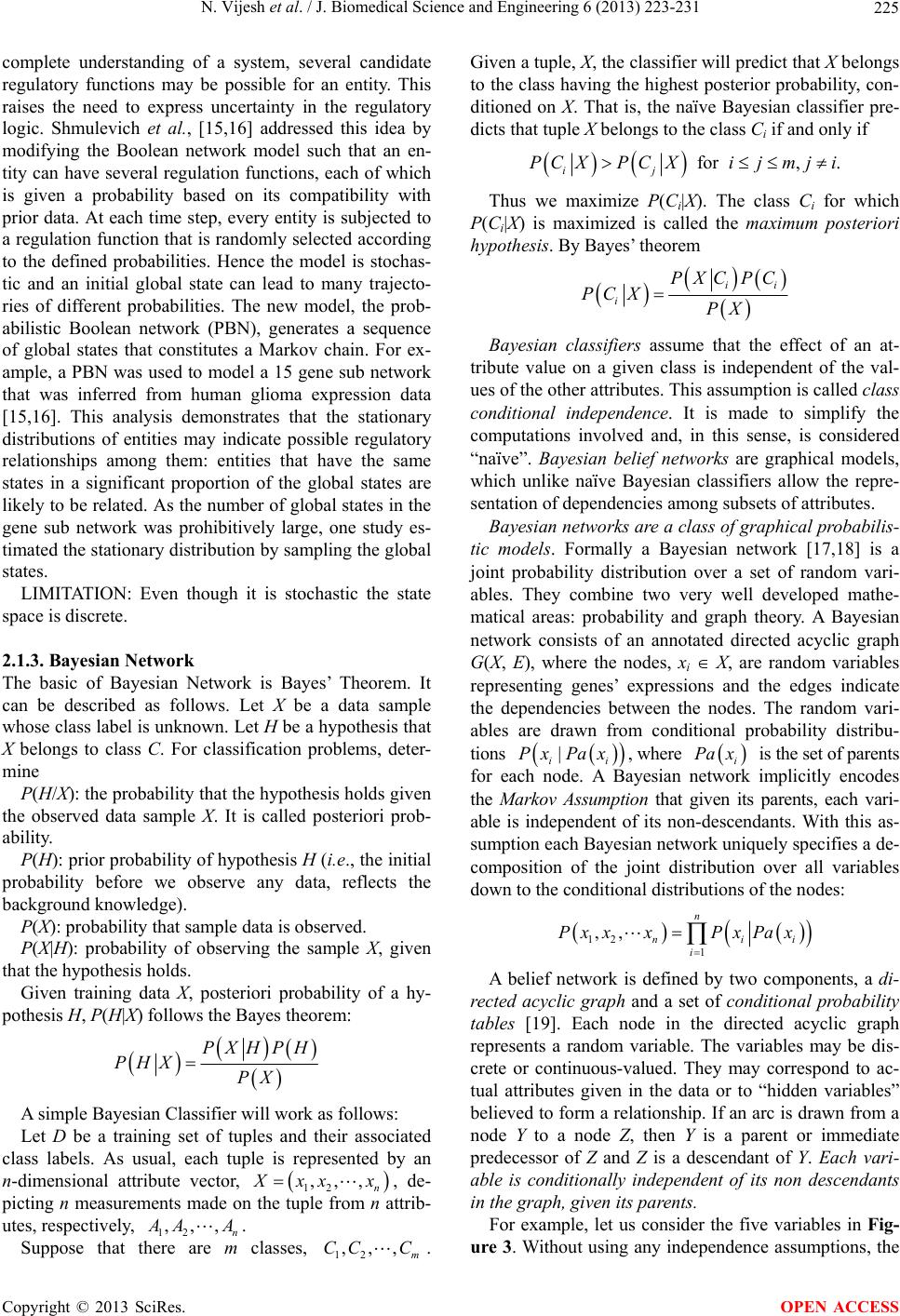 N. Vijesh et al. / J. Biomedical Science and Engineering 6 (2013) 223-231 225 complete understanding of a system, several candidate regulatory functions may be possible for an entity. This raises the need to express uncertainty in the regulatory logic. Shmulevich et al., [15,16] addressed this idea by modifying the Boolean network model such that an en- tity can have several regulation functions, each of which is given a probability based on its compatibility with prior data. At each time step, every entity is subjected to a regulation function that is randomly selected according to the defined probabilities. Hence the model is stochas- tic and an initial global state can lead to many trajecto- ries of different probabilities. The new model, the prob- abilistic Boolean network (PBN), generates a sequence of global states that constitutes a Markov chain. For ex- ample, a PBN was used to model a 15 gene sub network that was inferred from human glioma expression data [15,16]. This analysis demonstrates that the stationary distributions of entities may indicate possible regulatory relationships among them: entities that have the same states in a significant proportion of the global states are likely to be related. As the number of global states in the gene sub network was prohibitively large, one study es- timated the stationary distribution by sampling the global states. LIMITATION: Even though it is stochastic the state space is discrete. 2.1.3. Bayesian Network The basic of Bayesian Network is Bayes’ Theorem. It can be described as follows. Let X be a data sample whose class label is unknown. Let H be a hypothesis that X belongs to class C. For classification problems, deter- mine P(H/X): the probability that the hypothesis holds given the observed data sample X. It is called posteriori prob- ability. P(H): prior probability of hypothesis H (i.e., the initial probability before we observe any data, reflects the background knowledge). P(X): probability that sample data is observed. P(X|H): probability of observing the sample X, given that the hypothesis holds. Given training data X, posteriori probability of a hy- pothesis H, P(H|X) follows the Bayes theorem: PXHPH PHX PX A simple Bayesian Classifier will work as follows: Let D be a training set of tuples and their associated class labels. As usual, each tuple is represented by an n-dimensional attribute vector, 12 ,,, n xx x, de- picting n measurements made on the tuple from n attrib- utes, respectively, 12 ,,, n AA. Suppose that there are m classes, . Given a tuple, X, the classifier will predict that X belongs to the class having the highest posterior probability, con- ditioned on X. That is, the naïve Bayesian classifier pre- dicts that tuple X belongs to the class Ci if and only if 12 , m C,,CC for, . ij PCXPCXij mj i Thus we maximize P(Ci|X). The class Ci for which P(Ci|X) is maximized is called the maximum posteriori hypothesis. By Bayes’ theorem ii i PXC PC PC XPX Bayesian classifiers assume that the effect of an at- tribute value on a given class is independent of the val- ues of the other attributes. This assumption is called class conditional independence. It is made to simplify the computations involved and, in this sense, is considered “naïve”. Bayesian belief networks are graphical models, which unlike naïve Bayesian classifiers allow the repre- sentation of dependencies among subsets of attributes. Bayesian networks are a class of graphical probabilis- tic models. Formally a Bayesian network [17,18] is a joint probability distribution over a set of random vari- ables. They combine two very well developed mathe- matical areas: probability and graph theory. A Bayesian network consists of an annotated directed acyclic graph G(X, E), where the nodes, xi X, are random variables representing genes’ expressions and the edges indicate the dependencies between the nodes. The random vari- ables are drawn from conditional probability distribu- tions | ii xPax, where i Pa x is the set of parents for each node. A Bayesian network implicitly encodes the Markov Assumption that given its parents, each vari- able is independent of its non-descendants. With this as- sumption each Bayesian network uniquely specifies a de- composition of the joint distribution over all variables down to the conditional distributions of the nodes: 12 1 ,, n ni i Px xxPxPax i A belief network is defined by two components, a di- rected acyclic graph and a set of conditional probability tables [19]. Each node in the directed acyclic graph represents a random variable. The variables may be dis- crete or continuous-valued. They may correspond to ac- tual attributes given in the data or to “hidden variables” believed to form a relationship. If an arc is drawn from a node Y to a node Z, then Y is a parent or immediate predecessor of Z and Z is a descendant of Y. Each vari- able is conditionally independent of its non descendants in the graph, given its parents. For example, let us consider the five variables in Fig- ure 3. Without using any independence assumptions, the Copyright © 2013 SciRes. OPEN ACCESS  N. Vijesh et al. / J. Biomedical Science and Engineering 6 (2013) 223-231 226 Figure 3. Conditional independence in a sim- ple Bayesian network. This network structure implies several condi- tional independence ⊥⊥ cases: (A E), (B ⊥ D | A, E), (C A, D, ⊥ E | B), (D B, C, E | ⊥ A), and (E A, D). joint probability distribution can be written as: ,,,,,,, ,, , PABCDEP EABCD P DABC PCABPBAPA . In contrast, using the independence assumptions im- plied by the network in Figure 3, the same distribution can be expressed as: ,,, ,,PABCDE PEPAPBAEPDAPCB. If the variables are all binary in this network, the former form requires 31 parameters, while the latter only needs 10 parameters. More generally, if G is defined over N binary variables and their maximal number of parents is bound by M, then instead of using 2N − 1 independent parameters to represent the full joint probability distribu- tion, a Bayesian network model can represent the same joint distribution with at most 2MN parameters. A node within the network can be selected as an “out- put” node, representing a class label attribute. There may be more than one output node. Various algorithms for learning can be applied to the network. Rather than re- turning a single class label, the classification process can return a probability distribution that gives the probability of each class. A major advantage of Bayesian network models is the ability to learn them from observed data. Bayesian networks can capture linear, non-linear, com- binatorial, stochastic and other types of relationships among variables. They are suitable for modeling gene networks because of their ability to represent stochastic events, to describe locally interacting processes, to han- dle noisy or missing biological data in a principled statis- tical way and to possibly make causal inferences from the derived models [20,21]. Hence, Bayesian networks, including their variants Dynamic Bayesian networks, Gaussian networks, Module networks, mixture Bayesian networks and state-space models (SSMs), etc., have be- come widely used tools for regulatory-network model- ing. LIMITATION: Although effective in dealing with noise, incompleteness and stochastic aspects of gene regulation, they fail to consider temporal dynamic as- pects that are an important part of regulatory networks modeling. Dynamic Bayesian networks (DBN) evolved feedback loops to effectively deal with the temporal as- pects of regulatory networks but their benefits are hin- dered by the high computational cost required for learn- ing the conditional dependencies in the cases where large numbers of genes are involved. 2.2. Continuous Models Biological experiments usually produce real, rather than discrete valued, measurements. Examples include reac- tion rates, cell mass [22-25], cell cycle length and gene expression intensities. Logical models require discretiza- tion of the real valued data, which reduces the accuracy of the data. Continuous models, using real valued pa- rameters over a continuous timescale, allow a straight- forward comparison of the global state and experimental data and can theoretically be more accurate. In practice, however, quantitative measurements are almost always partial (that is, they cover only a fraction of the system’s entities). Therefore, some of the parameters of continu- ous models are usually based on estimations or inference. 2.2.1. Linear Model The defining property of linear models is that each regu- lator contributes to the input of the regulation function independently of the other regulators, in an additive manner [10]. In other words, the change in the level of each entity depends on a weighted linear sum of the lev- els of its regulators. This assumption allows a high level of abstraction and efficient inference of network struc- ture and regulation functions. A biological system can be considered to be a state machine, where the change in internal state of the system depends on the current internal state plus any external inputs. The mRNA levels form an important part of the internal state of a cell (ideally, we also want to measure protein levels, metabolites, etc.). As a first approximation, we fit the expression data with a purely linear model, where the change in expression level of each mRNA species is derived as a weighted sum of the expression levels of all other genes. Of course, a linear model can never be much more than a caricature of the real system, but perhaps we can still draw some interesting conclu- sions from it. The basic linear model is of the form ii j jj tt WXt , where Xi(t + Δt) is the expression level of gene i at time t + Δt, and Wij indicates how much the level of gene j inu- Copyright © 2013 SciRes. OPEN ACCESS  N. Vijesh et al. / J. Biomedical Science and Engineering 6 (2013) 223-231 227 ences gene i. For each gene, we will also add an extra term indicating the influence of kainate, and a constant bias term to model the activation level of the gene in the absence of any other regulatory inputs. The differences in gene regulation due to tissue type will be modeled by a difference in bias. The final formula becomes: kainat e iijji jii tt WXtKtCT where kainate(t) is the kainate level at time t, Ki is the influence of kainate on gene i, Ci is a constant bias factor for each gene, and Ti indicates the difference in bias be- tween tissue types (Ti = 0 when simulating spinal cord, so the total bias for spinal cord is Ci, for hippocampus Ci + Ti). LIMITATION: Linear additive regulation models re- vealed certain linear relations in regulatory systems but failed to capture nonlinear dynamics aspects of genes regulation. When higher sensitivity to detail is desired, more complex models are preferable. 2.2.2. Differential Equ a ti on B ased M odel Differential equation models encode a gene network as a system of differential equations. Difference and differen- tial equations allow more detailed descriptions of net- work dynamics, by explicitly modelling the concentra- tion changes of molecules over time [26,27]. The basic difference equation model is of the form 111111 11 nn nnnnnn ttgt wgtwgtt tt gtwgtwgtt where gi(t + Δt) is the expression level of gene i at time t + Δt, and wij the weight indicating how much the level of gene i is influenced by gene j ,1,,ij n. Note that this model assumes a linear logic control model—the expression levels of genes at a time t + Δt, depends line- arly on the expression levels of all genes at a time t. For each gene, one can add extra terms indicating the influ- ence of additional substances. Differential equation mo- dels are similar to difference equation models, but follow concentration changes continuously, modelling the time difference between two time steps in infinitely small time increases, i.e. Δt is approaching 0. Difference and differential models depend on numeri- cal parameters, which are often difficult to measure ex- perimentally. An important question for these models is stability—does the behaviour of the system depend on the exact values of these parameters and initial substance concentrations, or is it similar for different variations. It seems unlikely that an unstable system represents a bio- logically realistic model, while on the other hand, if the system is stable, the exact values of some parameters may not be essential. The rate of change in concentration of a particular transcript is given by an influence function of other RNA concentrations. The non-linear differential equations de- scribe the mutual activating and repressing influences of genes in a GRN at a high-level of abstraction. In particu- lar, it is assumed that the rate of gene expression depends exclusively on the concentration of gene products arising from the nodes (genes) of the GRN. This means that the influence of other molecules (e.g., transcription factors) and cellular processes (translation) is not taken into ac- count directly. Even with these limitations, dynamic GRN models of this kind can be useful in deciphering basic aspects of gene-regulatory interactions. One major advantage of all three methods described below lies in their simple homogeneous structures, as this allows the settings of parameter discovering software to be easily customized for these structures. The three methods describe dynamic GRN models by means of a system (or set) of ordinary differential equations. For a GRN comprising N genes, N differential equations are used to describe the dynamics of N gene product concen- trations, Xi with 1, ,iN . In all three methods, the expression rate dXi/dt of a gene product concentration may depend on the expression level of one or more gene products of the genes Xj, with . Thus, the gene product concentration Xi may be governed by a self-regulatory mechanism (when i = j), or it may be regulated by products of other genes in the GRN. The three modeling methods differ in the way they represent and calculate expression rates. 1, ,jN 2.2.2.1. The Artificial Neural Network (ANN) Method Vohradsky [28] introduced ANNs as a modeling method capable of describing the dynamic behavior of GRNs. The way this method represents and calculates expres- sion rates depends on the weighted sum of multiple regulatory inputs. This additive input processing is capa- ble of representing logical disjunctions. The expression rate is restricted to a certain interval where a sigmoidal transformation maps the regulatory input to the expres- sion interval. ANNs provide an additional external input which has an influence on this transformation in that it can regulate the sensitivity to the summed regulatory input. Finally, the ANN method defines the degradation of a gene product on the basis of standard mass-action kinetics. Formally, the ANN method is defined as: 1 d0 d N i iijjiiiiii j Xvf wXkXvk t The parameters of the ANN method have the follow- ing biological interpretations: N: Number of genes in the GRN to be modeled. The genes of the GRN are indexed by i and j, where ,1,,ij N . Copyright © 2013 SciRes. OPEN ACCESS  N. Vijesh et al. / J. Biomedical Science and Engineering 6 (2013) 223-231 228 vi: Maximal expression rate of gene i. wij: The connection weight or strength of control of gene j on gene i. Positive values of wij indicate activating influences while negative values define repressing influ- ences. ϑi: Influence of external input on gene i, which modu- lates the gene’s sensitivity of response to activating or repressing influences. f: Represents a non-linear sigmoid transfer function modifying the influence of gene expression products Xj and external input ϑi to keep the activation from growing without bounds. ki: Degradation of the i-th gene expression product. The mathematical properties of the ANN method have been well studied because it is a special case of a recur- rent neural network. In particular, the symmetry of the matrix of connection weights wij influences whether the network dynamics are oscillatory or whether they con- verge on a steady (or even chaotic) state. High positive or negative values of the external input, ϑi, reduce the effect of the connection weights. This is explored in Case D where ϑi has been interpreted as a delay to the reaction kinetics of the transcriptional machinery. 2.2.2.2. The S-System (SS) Method Savageau [29] proposed the synergistic system or S-system (SS) as a method to model molecular networks. When modeling GRNs with the SS method, the expres- sion rates are described by the difference of two products of power-law functions, where the first represents the activation term and the second the degradation term of a gene product Xi. This multiplicative input processing can be used to define logical conjunctions for both the regu- lation of gene expression processes and for the regulation of degradation processes. The SS method has no restric- tions in the gene expression rates and thus does not im- plicitly describe saturation. Formally, the SS method is defined as: 11 d,0,, d ij ij NN gh i ijijii ijij jj XXX gh t R R The parameters of the SS method have the following biological interpretations: N: Number of genes in the GRN to be modeled. The genes of the GRN are indexed by i and j, where . ,1,,ij N αi: Rate constant of activation term; in SS GRN mod- els, all activation (up-regulation) processes of a gene i are aggregated into a single activation term. βi: Rate constant of degradation term; in SS GRN models, all degradation processes of a gene i are aggre- gated into a single degradation term. gij,hij: Exponential parameters called kinetic order. These parameters describe the interactive influences of gene j on gene i. Positive values of gij indicate an acti- vating influence on the expression of gene i, whereas inhibiting influences are represented by negative values. Similarly, positive values of hij indicate increasing deg- radation of the gene product Xi, whereas decreasing deg- radation is represented by negative values. The parame- ters used in SS models have a clear physical meaning and can be measured experimentally, yet they describe phenomenological influences, as opposed to stoichio- metric rate constants in general mass action (GMA) sys- tems. The SS method generalizes mass-action kinetics by aggregating all individual processes into a single activi- tion and a single degradation term (per gene). In contrast, the GMA system defines all individual processes k with 1, ,k with the sum of power-law functions ac- cording to: 11 11 d d ,0,, ijk ijk NN RR gh i ik jik j kk jj ikikijk ijk XXX t gh R The parameters of the GMA system have the follow- ing biological interpretations: αi: Rate constant of activation process k. βik: Rate constant of degradation process k. gijk: Exponential parameter called kinetic order de- scribing the interactive influence of Xj on gene i of proc- ess k. hijk: Exponential parameter called kinetic order de- scribing the interactive influence of Xj on gene i of proc- ess k. 2.2.2.3. The General Rate Law of Transcription (GRLOT) Method The GRLOT method has been used to generate bench- mark time-series data sets to facilitate the evaluation of different reverse-engineering approaches. GRLOT mod- els multiply individual regulatory inputs. Activation and inhibition are represented by different functional expres- sions that are similar to Hill kinetics, which allow the inclusion of cooperative binding events. Identical to the ANN, the degradation of gene products is defined via mass-action kinetics. Formally, the GRLOT method is defined as: d d ,, ,0. jk jjk k nn j ik ii nnn n jk kk jj ij ji Ki XA vk tAKa IKi vKi Kak i X The parameters of the GRLOT method have the fol- lowing biological interpretations: vi: Maximal expression rate of gene i. Ij: Inhibitor (repressor) j. Ak: Activator k; the number of inhibitors I, and the Copyright © 2013 SciRes. OPEN ACCESS 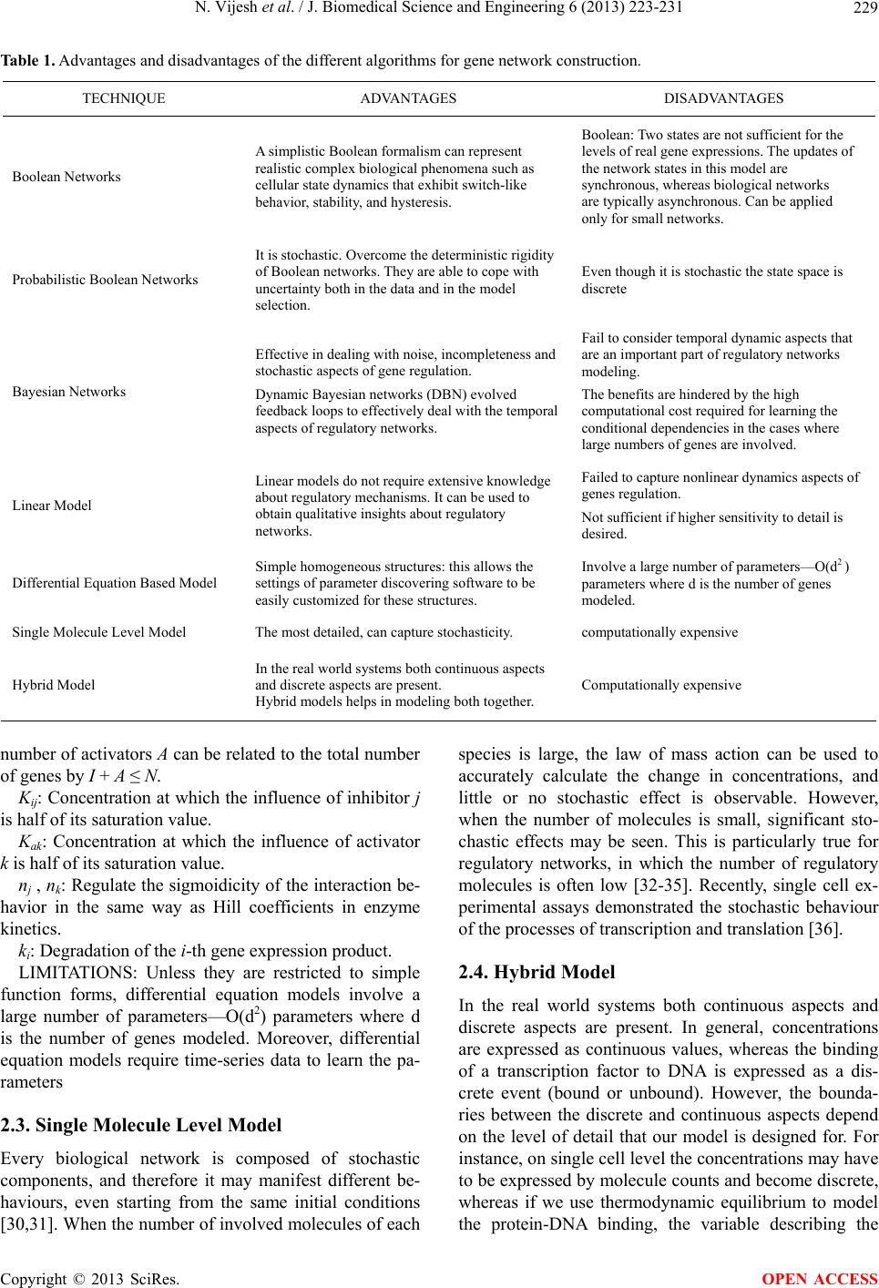 N. Vijesh et al. / J. Biomedical Science and Engineering 6 (2013) 223-231 Copyright © 2013 SciRes. 229 OPEN ACCESS Table 1. Advantages and disadvantages of the different algorithms for gene network construction. TECHNIQUE ADVANTAGES DISADVANTAGES Boolean Networks A simplistic Boolean formalism can represent realistic complex biological phenomena such as cellular state dynamics that exhibit switch-like behavior, stability, and hysteresis. Boolean: Two states are not sufficient for the levels of real gene expressions. The updates of the network states in this model are synchronous, whereas biological networks are typically asynchronous. Can be applied only for small networks. Probabilistic Boolean Networks It is stochastic. Overcome the deterministic rigidity of Boolean networks. They are able to cope with uncertainty both in the data and in the model selection. Even though it is stochastic the state space is discrete Bayesian Networks Effective in dealing with noise, incompleteness and stochastic aspects of gene regulation. Dynamic Bayesian networks (DBN) evolved feedback loops to effectively deal with the temporal aspects of regulatory networks. Fail to consider temporal dynamic aspects that are an important part of regulatory networks modeling. The benefits are hindered by the high computational cost required for learning the conditional dependencies in the cases where large numbers of genes are involved. Linear Model Linear models do not require extensive knowledge about regulatory mechanisms. It can be used to obtain qualitative insights about regulatory networks. Failed to capture nonlinear dynamics aspects of genes regulation. Not sufficient if higher sensitivity to detail is desired. Differential Equation Based Model Simple homogeneous structures: this allows the settings of parameter discovering software to be easily customized for these structures. Involve a large number of parameters—O(d2 ) parameters where d is the number of genes modeled. Single Molecule Level Model The most detailed, can capture stochasticity. computationally expensive Hybrid Model In the real world systems both continuous aspects and discrete aspects are present. Hybrid models helps in modeling both together. Computationally expensive number of activators A can be related to the total number of genes by I + A ≤ N. Kij: Concentration at which the influence of inhibitor j is half of its saturation value. Kak: Concentration at which the influence of activator k is half of its saturation value. nj , nk: Regulate the sigmoidicity of the interaction be- havior in the same way as Hill coefficients in enzyme kinetics. ki: Degradation of the i-th gene expression product. LIMITATIONS: Unless they are restricted to simple function forms, differential equation models involve a large number of parameters—O(d2) parameters where d is the number of genes modeled. Moreover, differential equation models require time-series data to learn the pa- rameters 2.3. Single Molecule Level Model Every biological network is composed of stochastic components, and therefore it may manifest different be- haviours, even starting from the same initial conditions [30,31]. When the number of involved molecules of each species is large, the law of mass action can be used to accurately calculate the change in concentrations, and little or no stochastic effect is observable. However, when the number of molecules is small, significant sto- chastic effects may be seen. This is particularly true for regulatory networks, in which the number of regulatory molecules is often low [32-35]. Recently, single cell ex- perimental assays demonstrated the stochastic behaviour of the processes of transcription and translation [36]. 2.4. Hybrid Model In the real world systems both continuous aspects and discrete aspects are present. In general, concentrations are expressed as continuous values, whereas the binding of a transcription factor to DNA is expressed as a dis- crete event (bound or unbound). However, the bounda- ries between the discrete and continuous aspects depend on the level of detail that our model is designed for. For instance, on single cell level the concentrations may have to be expressed by molecule counts and become discrete, whereas if we use thermodynamic equilibrium to model the protein-DNA binding, the variable describing the  N. Vijesh et al. / J. Biomedical Science and Engineering 6 (2013) 223-231 230 binding state becomes continuous. Hybrid models have been developed in an attempt to describe both, discrete and continuous aspects in one model. An example of a hybrid model [37,38] is a multi-layer evolutionary trained neuro-fuzzy recurrent network (ENFRN) applied to the problem of GRN reconstruction, which addresses the major drawbacks of currently exist- ing computational methods. This choice was driven by the benefits, in terms of computational power, that neural network based methods provide. The self-organized na- ture of ENFRN algorithm is able to produce an adaptive number of temporal fuzzy rules that describe the rela- tionships between the input (regulating) genes and the output (regulated) gene. Related to that, another advan- tage of this approach is that it overcomes the need of prior data discretization, a characteristic of many com- putational methods which often leads to information loss. The dynamic mapping capabilities emerging from the recurrent structure of ENFRN and the incorporation of fuzzy logic drive the construction of easily interpretable fuzzy rules of the form: “IF gene x is highly expressed at time t THEN its dependent/target gene y will be lowly expressed at time t + 1”. The evolutionary training, based on the PSO framework, tries to avoid the drawbacks of classical neural networks training algorithms [39]. Addi- tionally, we are approaching the under-determinism pro- blem by selecting the most suitable set of regulatory genes via a time-effective procedure embedded in the construction phase of ENFRN. Also, besides determining the regulatory relations among genes, this method can determine the type of the regulation (activation or re- pression) and at the same time assign a score, which might be used as a measure of confidence in the retrieved regulation. Comparison of different models discussed in this pa- per is given in Table 1. 3. CONCLUSION In this paper we have reviewed the different modeling methods for reconstructing gene networks from gene expression data. All methods mentioned above are for reverse engineering of GRNs from gene expression data. The Boolean network models have the limitation of dis- crete apace and in reality, of course, the levels of gene expression do not have only two states but can assume virtually continuous values. The probabilistic methods have the flexibility of assuming different probability of expression for gene at a particular point of time and are closely related to real time situations. Also we discussed continuous models like linear and differential models using non-discrete values. Single molecule based models consider stochastic behavior of biological network and hybrid models combines different concepts for GRN reconstruction. 4. ACKNOWLEDGEMENTS The authors wish to acknowledge the financial support provided by Department of Information Technology (DIT) Government of India for carrying out this work. REFERENCES [1] Guy, K. and Ron, S. (2008) Modelling and analysis of gene regulatory networks. www.nature.com/reviews/molcellbio [2] Davidson, E. and Levin, M. (2005) Gene regulatory net- works. Proceedings of the National Academy of Sciences of the United States of America, 102, 4935. doi:10.1073/pnas.0502024102 [3] Hasty, J., McMillen, D., Isaacs, F. and Collins, J.J. (2001) Computational studies of gene regulatory networks: In numero molecular biology. Nature Reviews Genetics, 2, 268-279. doi:10.1038/35066056 [4] Martin, T.S., Johannes, J.M. and Werner, D. (2010) Comparative study of three commonly used continuous deterministic methods for modeling gene regulation net- works. BMC Bioinformatics, 11, 459. doi:10.1186/1471-2105-11-459 [5] Wessels, L., van Someren, E. and Reinders, M.A. (3-7 January 2001) Comparison of genetic network models. Proceedings of the Pacific Symposium on Biocomputing, Hawaii, 508-519. [6] Cho, K.H., Choo, S.M., Jung, S.H., Kim, J.R., Choi, H.S., Kim, J. (2007) Reverse engineering of gene regulatory networks. IET Systems Biology, 1, 149-163. doi:10.1049/iet-syb:20060075 [7] De Jong, H. (2002) Modeling and simulation of genetic regulatory systems: A literature review. Journal of Com- putational Biology, 9, 67-103. doi:10.1089/10665270252833208 [8] Glass, L. and Kauffman, S.A. (1973) The logical analysis of continuous, non-linear biochemical control networks. Journal of Theoretical Biology, 39, 103-129. doi:10.1016/0022-5193(73)90208-7 [9] Thomas, R. (1973) Boolean formalization of genetic con- trol circuits. Journal of Theoretical Biology, 42, 563-585. doi:10.1016/0022-5193(73)90247-6 [10] Vladimir, F. (2005) Handbook of computational molecu- lar biology. University of California, Davis. [11] Faure, A., Naldi, A., Chaouiya, C. and Thieffry, D. (2006) Dynamical analysis of a generic boolean model for the control of the mammalian cell cycle. Bioinformatics, 22, e124-e131. doi:10.1093/bioinformatics/btl210 [12] Akutsu, T., Miyano, S. and Kuhara, S. (2000) Inferring quality relations in genetic networks and metabolic path- ways. Bioinformatics, 16, 727-734. doi:10.1093/bioinformatics/16.8.727 [13] Tany, A. and Shamir, R. (2001) Computational expansion of gene networks. Bioinformatics, 17, S270-S278. Copyright © 2013 SciRes. OPEN ACCESS  N. Vijesh et al. / J. Biomedical Science and Engineering 6 (2013) 223-231 Copyright © 2013 SciRes. 231 [27] D’Haeseleer, P., Wen, X., Fuhrman, S. and Somogyi, R. (1999) Linear modeling of mRNA expression levels dur- ing CNS development and injury. Pacific Symposium on Biocomputing, 4, 41-52. doi:10.1093/bioinformatics/17.suppl_1.S270 [14] Lahdesmaki, Shmuleveich, L. and Yli-Harja, O. (2003) On learning gene regulatory networks under the Boolean network model. Machine Learning, 52, 147-167. doi:10.1023/A:1023905711304 [28] Hellerstein, M.K. (2003) In vivo measurement of fluxes through metabolic pathways: The missing link in func- tional genomics and pharmaceutical research. Annual Re- view of Nutrition, 23, 379-402. doi:10.1146/annurev.nutr.23.011702.073045 [15] Shmulevich, I., Dougherty, E.R., Kim, S. and Zhang, W. (2002) Probabilistic Boolean networks: A rule-based un- certainty model for gene regulatory networks. Bioinfor- matics, 18, 261-274. doi:10.1093/bioinformatics/18.2.261 [29] Vohradsky, J. (2001) Neural network model of gene ex- pression. The FASEB Journal, 15, 846-854. doi:10.1096/fj.00-0361com [16] Shmulevich, I., Gluhovsky, I., Hashimoto, R.F., Dough- erty, E.R. and Zhan, W. (2003) Steady-state analysis of genetic regulatory networks modelled by probabilistic Boolean networks. Comparative and Functional Genom- ics, 4, 601-608. doi:10.1002/cfg.342 [30] Savageau, M.A. (1976) Biochemical systems analysis: A study of function and design in molecular biology. Addi- son-Wesley, Reading. [17] Pearl, J. (1988) Probabilistic reasoning in intelligent sys- tems: Networks of plausible inference. Morgan Kauf- mann, San Mateo. [31] McAdams, H.H. and Arkin, A. (1999) It’s a noisy busi- ness! Genetic regulation at the nanomolar scale. Trends in Genetics, 15, 65-69. doi:10.1016/S0168-9525(98)01659-X [18] Han, J.W. and Micheline, K. (2007) Data mining: Con- cepts and techniques. Elsevier Science, New York. [32] Ross, I.L., Browne, C.M. and Hume, D.A. (1994) Tran- scription of individual genes in eukaryotic cells occurs randomly and infrequently. Immunology & Cell Biology, 72, 177-185. doi:10.1038/icb.1994.26 [19] Friedman, N., Linial, M., Nachman, I. and Pe’er, D. (2000) Using Bayesian networks to analyze expression data. Journal of Computational Biology, 7, 601-620. doi:10.1089/106652700750050961 [33] Bae, K., Lee, C., Hardin, P.E. and Edery, I. (2000) dCLOCK is present in limiting amounts and likely medi- ates daily interactions between the dCLOCK-CYC tran- scription factor and the PER-TIM complex. Journal of Neuroscience, 20, 1746-1753. [20] Armaanzas, R., Inza, I. and Larraaga, P. (2008) Detecting reliable gene interactions by a hierarchy of Bayesian network classifiers. Computer Methods and Programs in Biomedicine, 91, 110-121. doi:10.1016/j.cmpb.2008.02.010 [34] Guptasarma, P. (1995) Does replication-induced tran- scription regulate synthesis of the myriad low copy num- ber proteins of Escherichia coli? Bioessays, 17, 987-997. doi:10.1002/bies.950171112 [21] Beal, M.J., Falciani, F., Ghahramani, Z., Rangel, C. and Wild, D.L. (2005) A Bayesian approach to reconstructing genetic regulatory networks with hidden factors. Bioin- formatics, 21, 349-356. doi:10.1093/bioinformatics/bti014 [35] Bailone, A., Levine, A. and Devoret, R. (1979) Inactiva- tion of prophage λ repressor in vivo. Journal of Molecular Biology, 131, 553-572. doi:10.1016/0022-2836(79)90007-X [22] Mason, O. and Verwoerd, M. (2007) Graph theory and networks in biology. IET Systems Biology, 1, 89-119. doi:10.1049/iet-syb:20060038 [36] Shea, M.A. and Ackers, G.K. (1985) The OR control system of bacteriophage λ. A physical-chemical model for gene regulation. Journal of Molecular Biology, 181, 211-230. doi:10.1016/0022-2836(85)90086-5 [23] Sauer, U., et al. (1996) Physiology and metabolic fluxes of wildtype and riboflavin-producing Bacillus subtilis. Applied and Environmental Microbiology, 62, 3687- 3696. [37] J. Paulsson. (2005) Models of stochastic gene expression. Physics of Life Reviews, 2, 157-175. doi:10.1016/j.plrev.2005.03.003 [24] Ness, S.A. (2006) Basic microarray analysis: Strategies for successful experiments. Methods in Molecular Biol- ogy, 316, 13-33. [38] Ioannis, A.M., Andrei, D. and Dimitris, T. (2010) Gene regulatory networks modelling using a dynamic evolu- tionary hybrid. BMC Bioinformatics, 11, 140. doi:10.1186/1471-2105-11-140 [25] Kingsmore, S.F. (2006) Multiplexed protein measure- ment: Technologies and applications of protein and anti- body arrays. Nature Reviews Drug Discovery, 5, 310-320. doi:10.1038/nrd2006 [39] Du, P., Gong, J., Wurtele, E.S. and Dickerson, J.A. (2005) Modeling gene expression networks using fuzzy logic. IEEE Transacions on Systems, Man and Cybernetics, 35, 1351-1359. doi:10.1109/TSMCB.2005.855590 [26] Chen, T., He, H.L. and Church, G.M. (1999) Modeling gene expression with differential equations. Pacific Sym- posium on Biocomputing, 4, 29-40. OPEN ACCESS
|