Treatment of Biased Error Distributions in SBAS

Paper Menu >>

Journal Menu >>

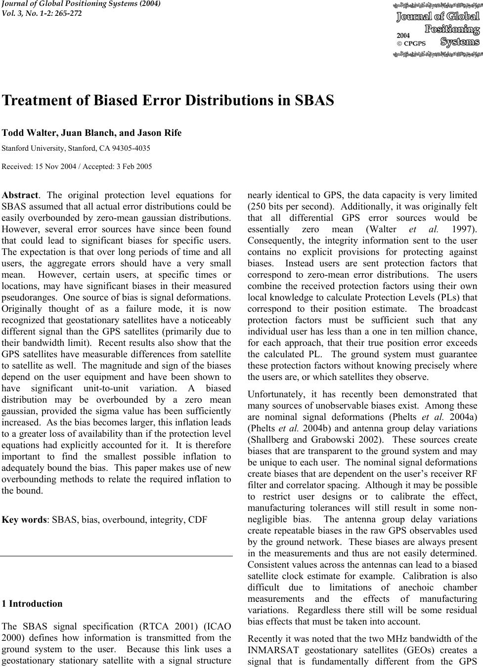Journal of Global Positioning Systems (2004)

Vol. 3, No. 1-2: 265-272

Treatment of Biased Error Distributions in SBAS

Todd Walter, Juan Blanch, and Jason Rife

Stanford University, Stanford, CA 94305-4035

Received: 15 Nov 2004 / Accepted: 3 Feb 2005

Abstract. The original protection level equations for

SBAS assumed that all actual error distributions could be

easily overbounded by zero-mean gaussian distributions.

However, several error sources have since been found

that could lead to significant biases for specific users.

The expectation is that over long periods of time and all

users, the aggregate errors should have a very small

mean. However, certain users, at specific times or

locations, may have significant biases in their measured

pseudoranges. One source of bias is signal deformations.

Originally thought of as a failure mode, it is now

recognized that geostationary satellites have a noticeably

different signal than the GPS satellites (primarily due to

their bandwidth limit). Recent results also show that the

GPS satellites have measurable differences from satellite

to satellite as well. The magnitude and sign of the biases

depend on the user equipment and have been shown to

have significant unit-to-unit variation. A biased

distribution may be overbounded by a zero mean

gaussian, provided the sigma value has been sufficiently

increased. As the bias becomes larger, this inflation leads

to a greater loss of availability than if the protection level

equations had explicitly accounted for it. It is therefore

important to find the smallest possible inflation to

adequately bound the bias. This paper makes use of new

overbounding methods to relate the required inflation to

the bound.

Key words: SBAS, bias, overbound, integrity, CDF

1 Introduction

The SBAS signal specification (RTCA 2001) (ICAO

2000) defines how information is transmitted from the

ground system to the user. Because this link uses a

geostationary stationary satellite with a signal structure

nearly identical to GPS, the data capacity is very limited

(250 bits per second). Additionally, it was originally felt

that all differential GPS error sources would be

essentially zero mean (Walter et al. 1997).

Consequently, the integrity information sent to the user

contains no explicit provisions for protecting against

biases. Instead users are sent protection factors that

correspond to zero-mean error distributions. The users

combine the received protection factors using their own

local knowledge to calculate Protection Levels (PLs) that

correspond to their position estimate. The broadcast

protection factors must be sufficient such that any

individual user has less than a one in ten million chance,

for each approach, that their true position error exceeds

the calculated PL. The ground system must guarantee

these protection factors without knowing precisely where

the users are, or which satellites they observe.

Unfortunately, it has recently been demonstrated that

many sources of unobservable biases exist. Among these

are nominal signal deformations (Phelts et al. 2004a)

(Phelts et al. 2004b) and antenna group delay variations

(Shallberg and Grabowski 2002). These sources create

biases that are transparent to the ground system and may

be unique to each user. The nominal signal deformations

create biases that are dependent on the user’s receiver RF

filter and correlator spacing. Although it may be possible

to restrict user designs or to calibrate the effect,

manufacturing tolerances will still result in some non-

negligible bias. The antenna group delay variations

create repeatable biases in the raw GPS observables used

by the ground network. These biases are always present

in the measurements and thus are not easily determined.

Consistent values across the antennas can lead to a biased

satellite clock estimate for example. Calibration is also

difficult due to limitations of anechoic chamber

measurements and the effects of manufacturing

variations. Regardless there still will be some residual

bias effects that must be taken into account.

Recently it was noted that the two MHz bandwidth of the

INMARSAT geostationary satellites (GEOs) creates a

signal that is fundamentally different from the GPS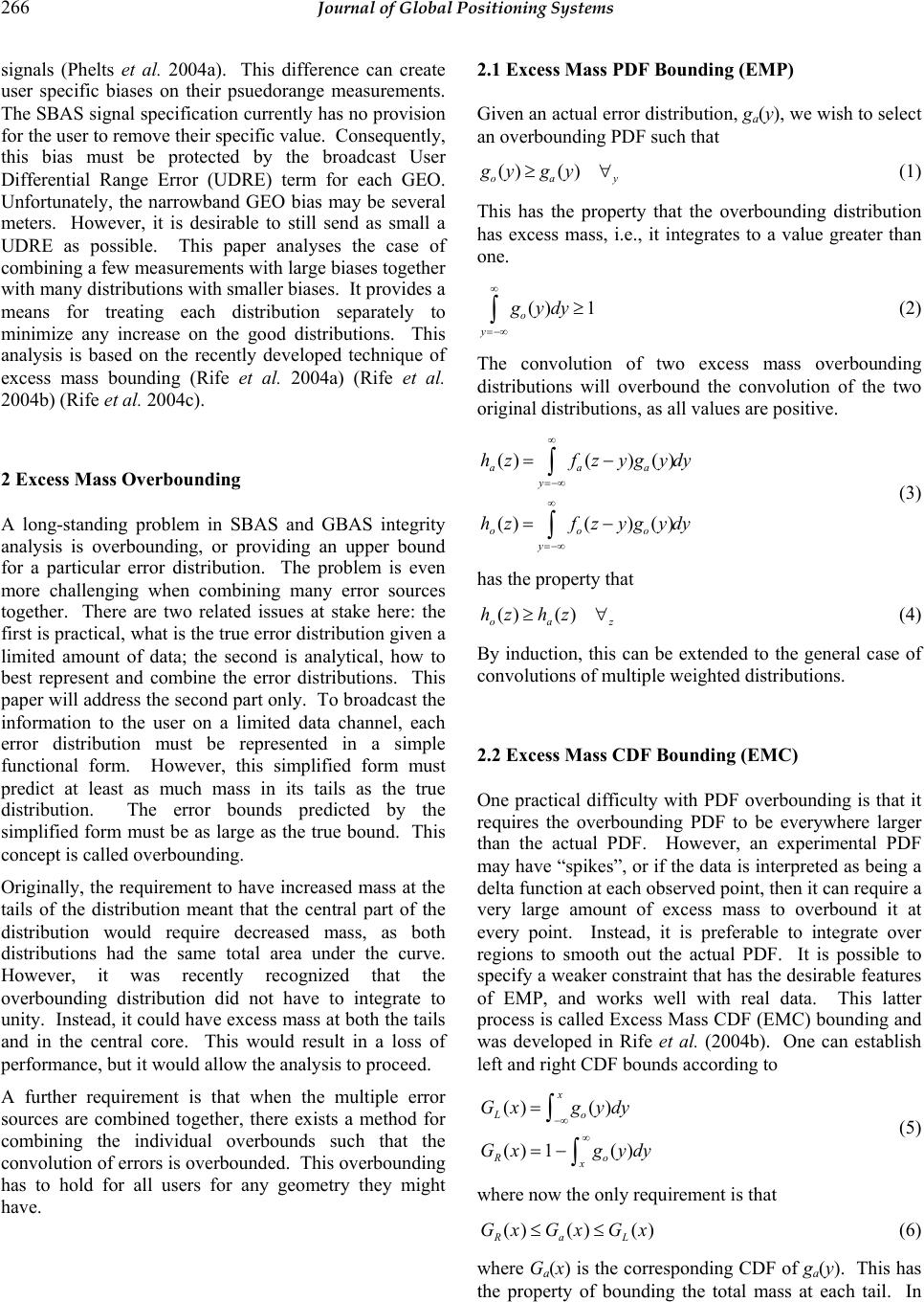

266 Journal of Global Positioning Systems

signals (Phelts et al. 2004a). This difference can create

user specific biases on their psuedorange measurements.

The SBAS signal specification currently has no provision

for the user to remove their specific value. Consequently,

this bias must be protected by the broadcast User

Differential Range Error (UDRE) term for each GEO.

Unfortunately, the narrowband GEO bias may be several

meters. However, it is desirable to still send as small a

UDRE as possible. This paper analyses the case of

combining a few measurements with large biases together

with many distributions with smaller biases. It provides a

means for treating each distribution separately to

minimize any increase on the good distributions. This

analysis is based on the recently developed technique of

excess mass bounding (Rife et al. 2004a) (Rife et al.

2004b) (Rife et al. 2004c).

2 Excess Mass Overbounding

A long-standing problem in SBAS and GBAS integrity

analysis is overbounding, or providing an upper bound

for a particular error distribution. The problem is even

more challenging when combining many error sources

together. There are two related issues at stake here: the

first is practical, what is the true error distribution given a

limited amount of data; the second is analytical, how to

best represent and combine the error distributions. This

paper will address the second part only. To broadcast the

information to the user on a limited data channel, each

error distribution must be represented in a simple

functional form. However, this simplified form must

predict at least as much mass in its tails as the true

distribution. The error bounds predicted by the

simplified form must be as large as the true bound. This

concept is called overbounding.

Originally, the requirement to have increased mass at the

tails of the distribution meant that the central part of the

distribution would require decreased mass, as both

distributions had the same total area under the curve.

However, it was recently recognized that the

overbounding distribution did not have to integrate to

unity. Instead, it could have excess mass at both the tails

and in the central core. This would result in a loss of

performance, but it would allow the analysis to proceed.

A further requirement is that when the multiple error

sources are combined together, there exists a method for

combining the individual overbounds such that the

convolution of errors is overbounded. This overbounding

has to hold for all users for any geometry they might

have.

2.1 Excess Mass PDF Bounding (EMP)

Given an actual error distribution, ga(y), we wish to select

an overbounding PDF such that

go(y)≥ga(y)

∀

y (1)

This has the property that the overbounding distribution

has excess mass, i.e., it integrates to a value greater than

one.

go(y)dy≥1

y=−∞

∞

∫ (2)

The convolution of two excess mass overbounding

distributions will overbound the convolution of the two

original distributions, as all values are positive.

ha(z)=fa(z−y)ga(y)

y=−∞

∞

∫dy

ho(z)=fo(z−y)go(y)

y=−∞

∞

∫dy

(3)

has the property that

ho(z)≥ha(z)

∀

z (4)

By induction, this can be extended to the general case of

convolutions of multiple weighted distributions.

2.2 Excess Mass CDF Bounding (EMC)

One practical difficulty with PDF overbounding is that it

requires the overbounding PDF to be everywhere larger

than the actual PDF. However, an experimental PDF

may have “spikes”, or if the data is interpreted as being a

delta function at each observed point, then it can require a

very large amount of excess mass to overbound it at

every point. Instead, it is preferable to integrate over

regions to smooth out the actual PDF. It is possible to

specify a weaker constraint that has the desirable features

of EMP, and works well with real data. This latter

process is called Excess Mass CDF (EMC) bounding and

was developed in Rife et al. (2004b). One can establish

left and right CDF bounds according to

GL(x)=go(y)dy

−∞

∫

GR(x)=1−go(y)dy

∞

∫ (5)

where now the only requirement is that

GR(x)

≤

Ga(x)

≤

GL(x) (6)

where Ga(x) is the corresponding CDF of ga(y). This has

the property of bounding the total mass at each tail. In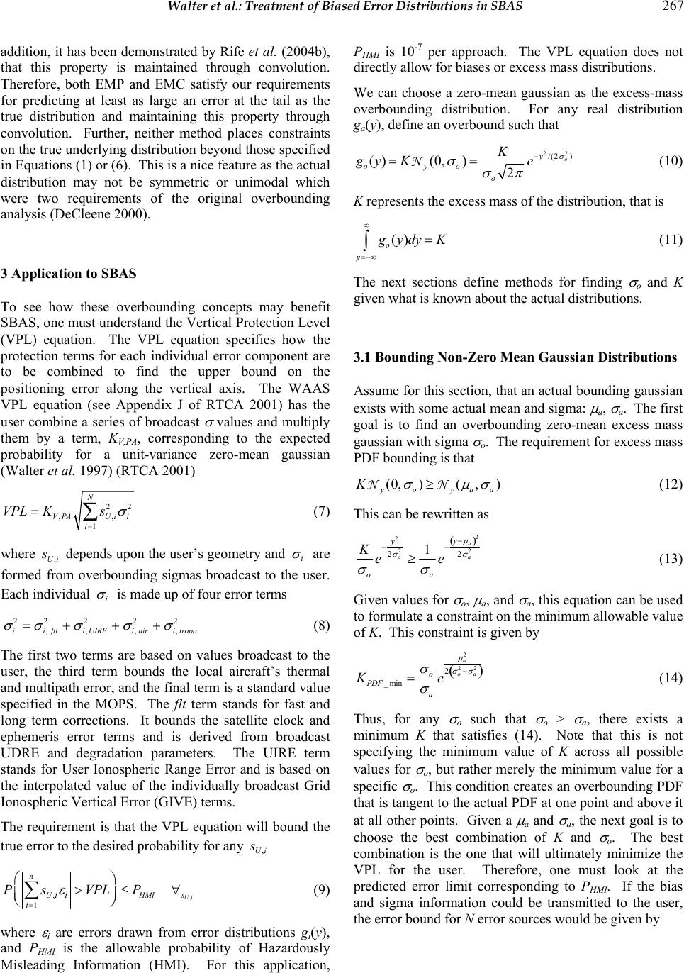

Walter et al.: Treatment of Biased Error Distributions in SBAS 267

addition, it has been demonstrated by Rife et al. (2004b),

that this property is maintained through convolution.

Therefore, both EMP and EMC satisfy our requirements

for predicting at least as large an error at the tail as the

true distribution and maintaining this property through

convolution. Further, neither method places constraints

on the true underlying distribution beyond those specified

in Equations (1) or (6). This is a nice feature as the actual

distribution may not be symmetric or unimodal which

were two requirements of the original overbounding

analysis (DeCleene 2000).

3 Application to SBAS

To see how these overbounding concepts may benefit

SBAS, one must understand the Vertical Protection Level

(VPL) equation. The VPL equation specifies how the

protection terms for each individual error component are

to be combined to find the upper bound on the

positioning error along the vertical axis. The WAAS

VPL equation (see Appendix J of RTCA 2001) has the

user combine a series of broadcast

values and multiply

them by a term, KV,PA, corresponding to the expected

probability for a unit-variance zero-mean gaussian

(Walter et al. 1997) (RTCA 2001)

VPL =KV,PA sU,i

i=1

∑ (7)

where sU,i depends upon the user’s geometry and

i are

formed from overbounding sigmas broadcast to the user.

Each individual

i is made up of four error terms

i,flt

i,UIRE

i,air

i,tropo

2 (8)

The first two terms are based on values broadcast to the

user, the third term bounds the local aircraft’s thermal

and multipath error, and the final term is a standard value

specified in the MOPS. The flt term stands for fast and

long term corrections. It bounds the satellite clock and

ephemeris error terms and is derived from broadcast

UDRE and degradation parameters. The UIRE term

stands for User Ionospheric Range Error and is based on

the interpolated value of the individually broadcast Grid

Ionospheric Vertical Error (GIVE) terms.

The requirement is that the VPL equation will bound the

true error to the desired probability for any sU,i

U,i

i=1

∑>VPL









≤P

HMI ∀sU,i (9)

where

i are errors drawn from error distributions gi(y),

and PHMI is the allowable probability of Hazardously

Misleading Information (HMI). For this application,

PHMI is 10-7 per approach. The VPL equation does not

directly allow for biases or excess mass distributions.

We can choose a zero-mean gaussian as the excess-mass

overbounding distribution. For any real distribution

ga(y), define an overbound such that

go(y)=KNy(0,

o)=K

e−y2/(2

2) (10)

K represents the excess mass of the distribution, that is

go(y)dy=K

y=−∞

∞

∫ (11)

The next sections define methods for finding

o and K

given what is known about the actual distributions.

3.1 Bounding Non-Zero Mean Gaussian Distributions

Assume for this section, that an actual bounding gaussian

exists with some actual mean and sigma:

a. The first

goal is to find an overbounding zero-mean excess mass

gaussian with sigma

o. The requirement for excess mass

PDF bounding is that

KNy(0,

o)≥Ny(

a) (12)

This can be rewritten as

−y2

2≥1

−y−

()

2 (13)

Given values for

a, and

a, this equation can be used

to formulate a constraint on the minimum allowable value

of K. This constraint is given by

KPDF _min =

2−

()

(14)

Thus, for any

o such that

o >

a, there exists a

minimum K that satisfies (14). Note that this is not

specifying the minimum value of K across all possible

values for

o, but rather merely the minimum value for a

specific

o. This condition creates an overbounding PDF

that is tangent to the actual PDF at one point and above it

at all other points. Given a

a and

a, the next goal is to

choose the best combination of K and

o. The best

combination is the one that will ultimately minimize the

VPL for the user. Therefore, one must look at the

predicted error limit corresponding to PHMI. If the bias

and sigma information could be transmitted to the user,

the error bound for N error sources would be given by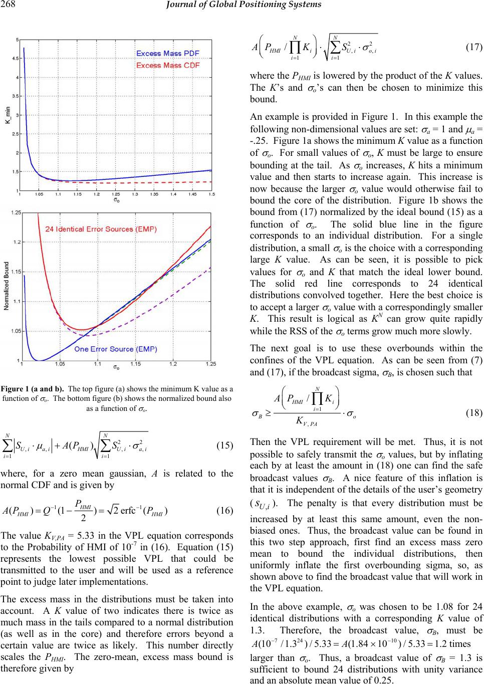

268 Journal of Global Positioning Systems

SU,i⋅

a,i

i=1

∑+A(P

HMI )SU,i

2⋅

a,i

i=1

∑ (15)

where, for a zero mean gaussian, A is related to the

normal CDF and is given by

A(P

HMI )=Q−1(1 −P

HMI

2)=2erfc−1(P

HMI ) (16)

The value KV,PA = 5.33 in the VPL equation corresponds

to the Probability of HMI of 10-7 in (16). Equation (15)

represents the lowest possible VPL that could be

transmitted to the user and will be used as a reference

point to judge later implementations.

The excess mass in the distributions must be taken into

account. A K value of two indicates there is twice as

much mass in the tails compared to a normal distribution

(as well as in the core) and therefore errors beyond a

certain value are twice as likely. This number directly

scales the PHMI. The zero-mean, excess mass bound is

therefore given by

HMI /Ki

i=1

∏









⋅SU,i

2⋅

o,i

i=1

∑ (17)

where the PHMI is lowered by the product of the K values.

The K’s and

o’s can then be chosen to minimize this

bound.

An example is provided in Figure 1. In this example the

following non-dimensional values are set:

a = 1 and

a =

-.25. Figure 1a shows the minimum K value as a function

o. For small values of

o, K must be large to ensure

bounding at the tail. As

o increases, K hits a minimum

value and then starts to increase again. This increase is

now because the larger

o value would otherwise fail to

bound the core of the distribution. Figure 1b shows the

bound from (17) normalized by the ideal bound (15) as a

function of

o. The solid blue line in the figure

corresponds to an individual distribution. For a single

distribution, a small

o is the choice with a corresponding

large K value. As can be seen, it is possible to pick

values for

o and K that match the ideal lower bound.

The solid red line corresponds to 24 identical

distributions convolved together. Here the best choice is

to accept a larger

o value with a correspondingly smaller

K. This result is logical as KN can grow quite rapidly

while the RSS of the

o terms grow much more slowly.

The next goal is to use these overbounds within the

confines of the VPL equation. As can be seen from (7)

and (17), if the broadcast sigma,

B, is chosen such that

B≥

HMI /Ki

i=1

∏











KV,PA

⋅

o (18)

Then the VPL requirement will be met. Thus, it is not

possible to safely transmit the

o values, but by inflating

each by at least the amount in (18) one can find the safe

broadcast values

B. A nice feature of this inflation is

that it is independent of the details of the user’s geometry

(sU,i). The penalty is that every distribution must be

increased by at least this same amount, even the non-

biased ones. Thus, the broadcast value can be found in

this two step approach, first find an excess mass zero

mean to bound the individual distributions, then

uniformly inflate the first overbounding sigma, so, as

shown above to find the broadcast value that will work in

the VPL equation.

In the above example,

o was chosen to be 1.08 for 24

identical distributions with a corresponding K value of

1.3. Therefore, the broadcast value,

B, must be

A(10 −7/1.3

24 )/ 5.33=A(1.84 ×10 −10 ) /5.33 =1.2 times

larger than

o. Thus, a broadcast value of

B = 1.3 is

sufficient to bound 24 distributions with unity variance

and an absolute mean value of 0.25.

Figure 1 (a and b). The top figure (a) shows the minimum K value as a

function of

o. The bottom figure (b) shows the normalized bound also

as a function of

Walter et al.: Treatment of Biased Error Distributions in SBAS 269

3.2 Applying Excess Mass CDF Bounding

The prior analysis used EMP bounding to derive

appropriate bounds. The requirement for excess mass

CDF bounding are analogous to (13) and can be written

in terms of the complimentary error function as

2erfc −x









≥1

2erfc −x+









∀x (19)

Although there is not a convenient closed form

expression for K, it can be found numerically from the

maximum value of the ratio

KCDF _min =max

erfc −x+











erfc −x























(20)

Against biased gaussian distributions, KCDF_min will

always be smaller than KPDF_min, although the difference

will be small. All of the remaining equations above will

work for EMC, except that a slightly smaller value for K

may be used. Figures 1 and 2 show the comparison of

the EMC vs. EMP. In Figure 1a, the EMC K value,

shown with the dashed line, is slightly smaller. This

improvement increases for larger values of

o. The main

difference is that the growth at larger

o values is

noticeably smaller. This is because the integration of the

mass at the tails is nearly sufficient to cover the core

distribution. In Figure 1b, the dashed lines represent the

bound from (17) normalized by the ideal bound (15) as a

function of

o for EMC. For the single source case

(dashed green line) there is little difference, both can

achieve the ideal bound (The CDF of the overbounds and

the actual distributions are tangent at 5.33). However, for

the 24 identical distribution case, there is a small

improvement. Now the optimal value of

o is closer to

1.09 and the bound is only about 4% greater than ideal

compared to 5% for EMP. Although EMC achieves

lower bounds and is more practical with real data, the rest

of this paper will continue to analyze EMP bounding.

This is because of the closed form equation possible with

EMP (14). It is worth remembering that this adds a small

amount of conservatism in the analysis. If one applied

EMC instead, one would have a small improvement.

This results in a small margin against integrity.

3.3 Validating Broadcast Values

In the WAAS safety analysis, the algorithms were

derived and then tested against real data. The data is used

to validate the performance of the algorithms. Because

the MOPS only allows discrete broadcast values for the

UDRE (14 numeric values) and GIVE (15 numeric

values), it is convenient to partition the data by

B. Thus,

rather than trying to find a

B value given a real

distribution, the important question becomes: Does the

chosen

B value sufficiently bound the actual histogram?

Because the feared biases are completely transparent to

the system, they are not present in the validation data.

Thus, the observed histograms are all nearly zero-mean.

The feared biases are bounded by separate analysis and

then included in this methodology. One can write that

the actual gaussian bounding parameters as fractions of

the desired broadcast value, that is:

Figure 2 (a and b). The top two graphs (a) show the PDF (upper) and

CDF (lower) for the two optimum cases in Figure 1b. The blue line

corresponds to the optimal single error source bound while the green

line is optimal for 24 identical distributions. The red line corresponds to

the actual distribution. The bottom two graphs (b) are the same plots

but on different scales to help see that the bounds (blue and green)

always stay above the red on the top plots, and to the left and right on

the bottom plots.

270 Journal of Global Positioning Systems

⋅

B (21)

where

is between 0 and 1. The notation in this paper is

slightly different from that in Rife et al. (2004c). This

paper looks in terms of reduction from the broadcast

value rather than inflation from the actual, thus

= 1/

From the histogram of data, it is possible to determine

values of

and K that bound the data. However,

will

be unobserved as the system will have removed known

biases. In Schempp and Rubin (2002) they determine

values for

(labelled

in their paper) for each of the

observed UDRE and GIVE values. The observed biases

are very small and can be treated as zero. The important

question is given the observed

’s how much margin is

there for unobserved biases? The goal is to find the

largest tolerable biases for given values of

It is useful to define

o also in terms of

B. From (18) it

can be seen that another parameter,

, can be defined

such that

⋅

≡KV,PA

HMI /Ki

i=1

∏











=KV,PA

2erfc−1P

HMI /Ki

i=1

∏











(22)

This parameter represents an upper bound on

. This

parameter is related to the

parameter in Rife et al.

(2004c) as

. As the product of the K’s increases,

so must the margin between

o and

B. Figure 3 shows a

plot of

versus the product of K’s. Fortunately, it is a

weak function and the product can grow quite large while

decreasing

by only a small amount.

To find a bound on

, Equation (14), can be rewritten as

KPDF _min =

2−

()

(23)

and inverted to yield

max =2

2−

()

ln KPDF _min









 (24)

However, KPDF_min depends on the other parameters. An

expression for it can be found by making a few other

assumptions. First, the product of the K’s can be

expressed as a function of

, by inverting its definition in

(22)

i=1

∏=P

HMI

erfc KV,PA











(25)

Next assume that the K product consists of two parts: a

fixed allocation for nearly zero mean distributions

(Kother), and a remainder that is evenly split among N

satellites. This is the key piece of the approach as it

allows for some satellites, such as the GEOs, to be treated

differently than the others. Then KPDF_min is given by

KPDF _min =P

HMI

erfc KV,PA









Kother













1/N

(26)

This value can be substituted into (24) to yield the final

expression for the maximum tolerable bias

max =2

2−

()

ln PHMI

erfc KV,PA









Kother













1/N













(27)

Since

is known from the histogram and PHMI, KV,PA and

Kother are fixed parameters, this function can be plotted

versus

to determine the maximum value.

An example is now provided to show how this process

may be used. WAAS has collected extensive data in

support of its certification in 2003 (Raytheon 2002). This

data has been examined in many ways, it has been found

that the largest

GPS for a particular

B is .65 (Schempp

2004) for GPS UDRE and GIVE values. The goal is to

determine the largest allowable bias on the GEO

satellites. For GPS and ionospheric error distributions,

allow K values up 1.15 to account for small biases and

other non-gaussian behaviour. Assuming a 12-channel

receiver and two narrowband GEOs, allows 22 GPS or

ionospheric induced errors and 2 GEO errors. The

parameter Kother is set to 1.1522 = 21.64. For the GEO the

GEO is either 0.7 for a minimum UDRE value of 7.5 m

or 0.35 for a minimum value of 15 m. Figure 4 shows the

results for setting Kother = 21.64 and

GEO = 0.7 (a) or

GEO = 0.35 (b), and assuming one or two GEO satellites.

Figure 3. The value

is shown as a function of the product of the K’s.

As can be seen it is a slow to decrease with very large K values.

Walter et al.: Treatment of Biased Error Distributions in SBAS 271

As can be seen from the figures, larger biases can be

tolerated for smaller

GEO values and for fewer numbers

of geostationary satellites. For the UDRE of 7.5 m (

B =

2.28 m) the maximum

value occurs near

= 0.8 and is

approximately 1.2 (

= 2.74 m) for one satellite, or 0.85

(

= 1.94 m) for two. For the UDRE floor of 15 m (

B =

4.56 m) the maximum

value occurs near

= 0.55 and is

approximately 3.3 (

= 15 m) for one satellite, or 2.3 (

10.49 m) for two. However, in the latter example,

cannot be allowed to go as low as 0.55 as

GPS must be

above 0.65. This additional constraint from the GPS

satellites implies that the lowest allowable

is about 0.7.

Thus, the true maximum biases for the UDRE floor of 15

m are approximately 2.9 (

= 13.22 m) for one satellite or

2.0 (

= 9.12 m) for two.

4. Conclusions

This paper took the concepts of excess mass bounding

and applied them specifically to the case when a few

biased error distributions are combined with many well-

behaved ones. Specifically the case for WAAS with two

narrowband GEOs was examined. It was shown that a

methodology exists for determining the maximum

tolerable bias under certain constraints. This

methodology shows that based on the WAAS validation

data, biases as large as 2.74 m can be tolerated for a GEO

UDRE value of 7.5 m, or as large as 13.22 m for a GEO

UDRE value of 15 m. These value decrease to 1.94 m

and 9.12 when two GEOs may be visible.

Excess mass bounding provides a methodology for

formally accounting for biases that may be present. This

methodology is fully compatible with the WAAS MOPS

VPL equation that is based on zero-mean gaussian error

distributions. CDF bounding in particular will work with

a wide variety of actual distributions that are non-zero

mean and non-gaussian. The methodology is also very

flexible in allowing certain distributions to be treated

differently from the others. Each distribution may be

bounded with unique K and

values. This method

allows for the accommodation of larger biases than

allowed by other methods.

Acknowledgements:

The authors would like to acknowledge the funding from

the FAA satellite navigation product team..

References

DeCleene B (2000) Defining pseudorange integrity –

overbounding, Proceedings of ION GPS 2000, Salt Lake

City, Utah, September

ICAO (2000) Annex 10 — Aeronautical

Telecommunications.Volume I (Radio Navigation Aids),

ICAO publication November 2000

Phelts RE, Walter T, Enge P, Akos DM, Shallberg K, and

Morrissey T (2004a) Range biases on the WAAS

geostationary satellites, Proceedings of the ION National

Technical Meeting, San Diego, California, 26-28 January

2004

Phelts RE (2004b) Nominal signal deformation: limits on GPS

range accuracy, Proceedings of the 2004 International

Symposium on GPS/GNSS, Sydney, Australia, 6-8

December

Raytheon (2002) Algorithm contribution to HMI for the wide

area augmentation system, Raytheon Company

Unpublished Work.

Figure 4 (a and b). The top figure (a) shows the maximum

value as a

function of

for two cases with

GEO = 0.7. The bottom figure (b)

shows the maximum

value as a function of

for two cases with

GEO = 0.35.

272 Journal of Global Positioning Systems

Rife J, Pullen S, Pervan B, and Enge P (2004a) Paired

overbounding and application to GPS augmentation,

Proceedings IEEE Position, Location and Navigation

Symposium, Monterey, California, April

Rife J, Pullen S, Pervan B, and Enge P (2004b) Core

overbounding and its implications for LAAS integrity,

Proceedings of ION GNSS 2004, Long Beach, California,

September

Rife J, Walter T, and Blanch J, (2004c) Overbounding SBAS

and GBAS error distributions with excess-mass

functions, Proceedings of the 2004 International

Symposium on GPS/GNSS, Sydney, Australia, 6-8

December

RTCA (2001) Minimum operational performance standards

for global positioning system/wide area augmentation

system airborne equipment, RTCA publication DO-229C.

Schempp TR and Rubin AL (2002) An application of Gaussian

overbounding for the WAAS fault free error analysis,

Proceedings of ION GPS 2002, Portland, Oregon, 24-27

September

Schempp TR (2004) A range domain bound on the GEO

unobservable bias, Raytheon Company unpublished work,

June 2004

Shallberg K and Grabowski J (2002) Considerations for

characterizing antenna induced range errors,

Proceedings of ION GPS 2002, Portland, Oregon, 24-27

September

Walter T, Enge P, and Hansen A (1997) A proposed integrity

equation for WAAS MOPS, Proceedings of ION GPS 97,

Kansas City, Missouri, 16-19 September