Accuracy Improvement of PLIC-VOF Volume-Tracking Method Using the Equation of Surface Normal Vector

doi:10.4236/apm.2013.31A031

Paper Menu >>

Journal Menu >>

Advances in Pure Mathematics, 2013, 3, 219-225

http://dx.doi.org/10.4236/apm.2013.31A031 Published Online January 2013 (http://www.scirp.org/journal/apm)

Accuracy Improvement of PLIC-VOF Volume-Tracking

Method Using the Equation of Surface Normal Vector

Mingyu Sun

Institute of Fluid Science, Tohoku University, Sendai, Japan

Email: sun.tohoku@gmail.com

Received November 13, 2012; revised December 14, 2012; accepted December 21, 2012

ABSTRACT

The PLIC/SN method that combines the second-order volume tracking method (PLIC-VOF) with the equation of sur-

face normal (SN) vector was recently proposed (M. Sun, “Volume Tracking of Subgrid Particles,” International Jour-

nal for Numerical Methods in Fluids, Vol. 66, No. 12, 2011, pp. 1530-1554). The method is able to track the motion of

a subgrid particle, but the accuracy is not as good as expected on high resolution grids for vortical flows. In this paper, a

simple unsplit multidimensional advection algorithm is coupled with the equation of SN vector. The advection algo-

rithm is formulated as the finite volume method, so that it can be used readily for both structured and unstructured grids

while maintaining the exact mass conservation. The new method improves the accuracy significantly for high resolution

grids. In the well-known test of the time-resolved vortex problem of T = 2, the circular interface is resolved with an

accuracy better than ever using the equation of SN vector.

Keywords: VOF; PLIC; PLIC/SN; Surface Normal; Interface; Level Set; Unstructured Grid

1. Introduction

The volume-of-fluid (VOF) is one of the most widely

used methods for the numerical simulation of interfacial

phenomena [1]. In the VOF method, the evolution of an

interface is predicted generally by solving the advection

equation



u (1)

where u is the velocity. Function



is the volume frac-

tion or color function at the discrete level. It is unity in a

cell filled with one phase, and is zero if the cell lies in the

other phase. Because the volume fraction is discontinu-

ous across a sharp interface, it is challenging to advect

(1). The volume tracking method, or geometric VOF

method, that resolves an interface basically within one

cell while maintaining the mass conservation, has been

developed for over decades [2,3]. In this method, the

interface in a cell is not tracked explicitly, but recon-

structed and approximated by a simple geometry, such as

simple line (piecewise constant) interface calculation

(SLIC) [4] and piecewise linear interface calculation

(PLIC). A historic review of the piecewise constant and

linear reconstructions can be found in [2,5]. In the PLIC,

the surface normal vector, n, is required to construct the

linear interface

0,hnr

(2)

where is the line constant. The normal vector can be

inferred from the spatial distribution of



, symbolically

by,





n (3)

A few numerical methods have been proposed for the

calculation of the surface normal from the volume frac-

tion directly by the finite-difference method [6], fitting

methods [7-10], or height function technique (e.g. [11]).

The difficulty that these methods must overcome is

originated from the discontinuous property of the volume

fraction. In fact, (3) is just a symbolic representation of

SN vector if



is interpreted as the discontinuous vol-

ume fraction. One may also integrate the same Equation

(1) for a smooth level-set function with the hope that its

gradient (3) can be straightforwardly evaluated with a

better accuracy, as proposed by Sussman and Puckett

[12].

Since it is the surface normal (3) instead of the level

set function itself that is required for the geometric VOF,

one may directly integrate the equation for the SN vec-

tors,







nun (4)

which can be readily derived by taking the gradient of (1).

Although the volume fraction is discontinuous, the SN

vector can be a continuous function near an interface, a

clear advantage for numerical analysis using the finite

difference method. Raessi et al. [13] investigated the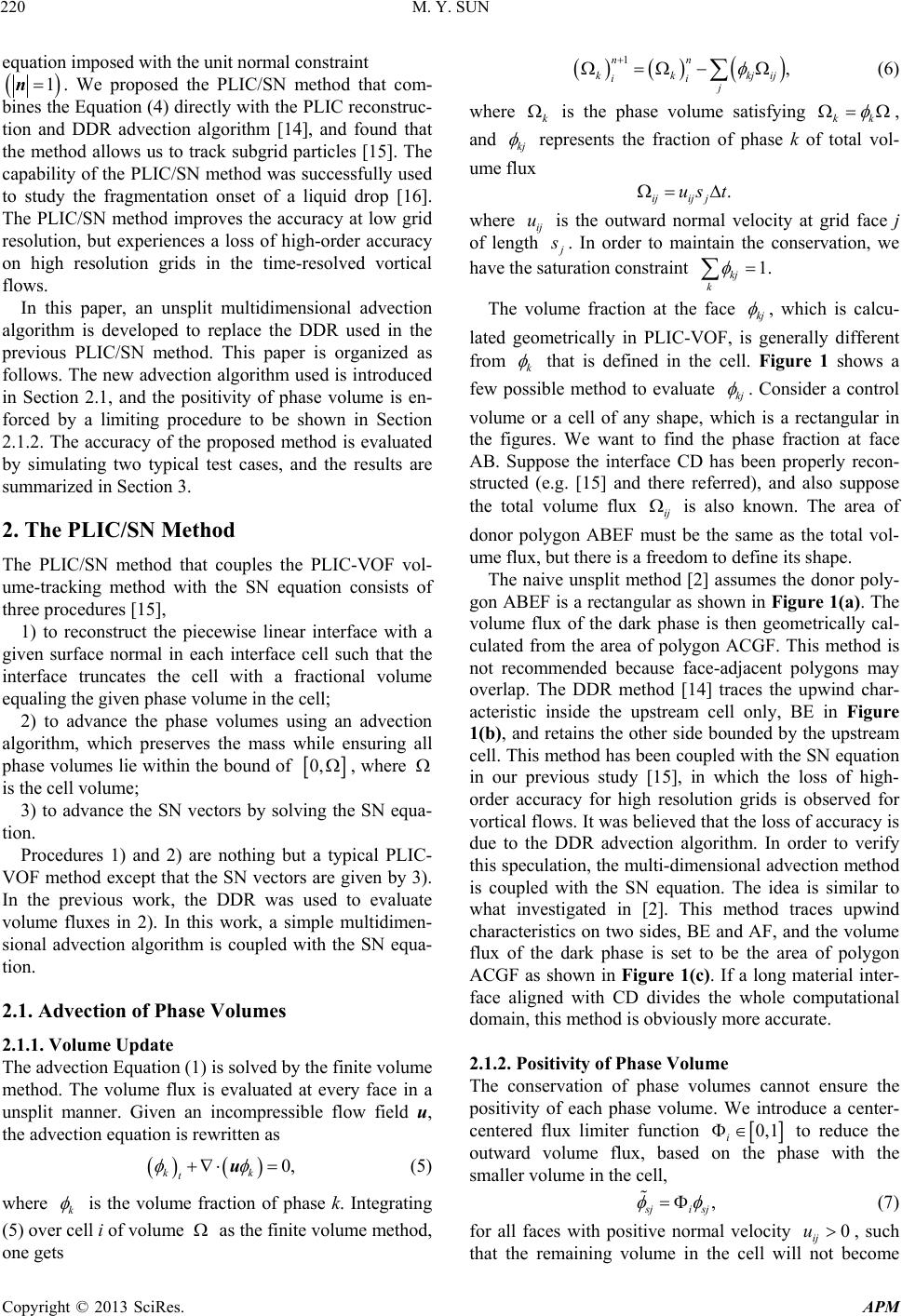

M. Y. SUN

220

equation imposed with the unit normal constraint



1n. We proposed the PLIC/SN method that com-

bines the Equation (4) directly with the PLIC reconstruc-

tion and DDR advection algorithm [14], and found that

the method allows us to track subgrid particles [15]. The

capability of the PLIC/SN method was successfully used

to study the fragmentation onset of a liquid drop [16].

The PLIC/SN method improves the accuracy at low grid

resolution, but experiences a loss of high-order accuracy

on high resolution grids in the time-resolved vortical

flows.

In this paper, an unsplit multidimensional advection

algorithm is developed to replace the DDR used in the

previous PLIC/SN method. This paper is organized as

follows. The new advection algorithm used is introduced

in Section 2.1, and the positivity of phase volume is en-

forced by a limiting procedure to be shown in Section

2.1.2. The accuracy of the proposed method is evaluated

by simulating two typical test cases, and the results are

summarized in Section 3.

2. The PLIC/SN Method

The PLIC/SN method that couples the PLIC-VOF vol-

ume-tracking method with the SN equation consists of

three procedures [15],

1) to reconstruct the piecewise linear interface with a

given surface normal in each interface cell such that the

interface truncates the cell with a fractional volume

equaling the given phase volume in the cell;

2) to advance the phase volumes using an advection

algorithm, which preserves the mass while ensuring all

phase volumes lie within the bound of





0,, where



is the cell volume;

3) to advance the SN vectors by solving the SN equa-

tion.

Procedures 1) and 2) are nothing but a typical PLIC-

VOF method except that the SN vectors are given by 3).

In the previous work, the DDR was used to evaluate

volume fluxes in 2). In this work, a simple multidimen-

sional advection algorithm is coupled with the SN equa-

tion.

2.1. Advection of Phase Volumes

2.1.1. Volume Update

The advection Equation (1) is solved by the finite volume

method. The volume flux is evaluated at every face in a

unsplit manner. Given an incompressible flow field u,

the advection equation is rewritten as









 u

t (5)

where



is the volume fraction of phase k. Integrating

(5) over cell i of volume as the finite volume method,

one gets



 



kkkjij





 



(6)

where



is the phase volume satisfying kk







and



represents the fraction of phase k of total vol-

ume flux

ijij j

us t





where ij is the outward normal velocity at grid face j

of length

. In order to maintain the conservation, we

have the saturation constraint







The volume fraction at the face



, which is calcu-

lated geometrically in PLIC-VOF, is generally different

from k



that is defined in the cell. Figure 1 shows a

few possible method to evaluate kj



. Consider a control

volume or a cell of any shape, which is a rectangular in

the figures. We want to find the phase fraction at face

AB. Suppose the interface CD has been properly recon-

structed (e.g. [15] and there referred), and also suppose

the total volume flux ij



is also known. The area of

donor polygon ABEF must be the same as the total vol-

ume flux, but there is a freedom to define its shape.

The naive unsplit method [2] assumes the donor poly-

gon ABEF is a rectangular as shown in Figure 1(a). The

volume flux of the dark phase is then geometrically cal-

culated from the area of polygon ACGF. This method is

not recommended because face-adjacent polygons may

overlap. The DDR method [14] traces the upwind char-

acteristic inside the upstream cell only, BE in Figure

1(b), and retains the other side bounded by the upstream

cell. This method has been coupled with the SN equation

in our previous study [15], in which the loss of high-

order accuracy for high resolution grids is observed for

vortical flows. It was believed that the loss of accuracy is

due to the DDR advection algorithm. In order to verify

this speculation, the multi-dimensional advection method

is coupled with the SN equation. The idea is similar to

what investigated in [2]. This method traces upwind

characteristics on two sides, BE and AF, and the volume

flux of the dark phase is set to be the area of polygon

ACGF as shown in Figure 1(c). If a long material inter-

face aligned with CD divides the whole computational

domain, this method is obviously more accurate.

2.1.2. Posi ti vi t y of Phase Volume

The conservation of phase volumes cannot ensure the

positivity of each phase volume. We introduce a center-

centered flux limiter function





0,1

i to reduce the

outward volume flux, based on the phase with the

smaller volume in the cell,

jisj







0u

(7)

for all faces with positive normal velocity ij , such

that the remaining volume in the cell will not become

M. Y. SUN 221

(a) (b)

(c)

Figure 1. Calculation of phase volume flux at face AB. Total

volume flux are the same for three cases, defined by the area

of ABEF. The volume flux of the dark phase is all given by

ACGF. (a) Naive unsplit advection method; (b) The DDR

method; (c) Multi-dim e n s i o n al advection metho d.

negative. The volume fraction of the other phase at the

face must be updated to 1







due to conservation.

A simple and efficient iterative method is used to cal-

culate . We start from the outward flux of the small

phase,



sj ij









f (8)

and then the first estimate of the limiter function can be

obtained by,



s,for

otherwise

f













(9)

where



 



, ,

is the volume of the small phase in the last

step. It can be easy shown that the small volume remains

non-negative if the phase volume is updated by using

limited flux (7). This limiter function was directly used

in [15].

In the initial estimate, only the outward volume fluxes

are considered, which leads to the strictest limiter func-

tion. The possible inward volume fluxes that increase the

volume are not considered. The limiter function may be

further relaxed by an iterative method. With the addi-

tional inward fluxes, (8) becomes,



,0 ,0

min

ij ij

sjij

ju ju











sj sjij











min,m

sj sj







(10)

and then i can be obtained similarly by (9). Super-

script m denotes the number of iterations. Notice that the

limiter function (7) tends to reduce the outward flux of

the small volume, and to increase that of the other large

volume due to conservation. Since the small phase in two

cell may be different, the inward flux is calculated by the

minimum possible flux, . Figure 2 re-

cords the geometrical errors in simulating a circular in-

terface in a time-resolved vortical velocity field, and the

details of this test will be introduced in Section 3. The

geometric error is reduced dramatically with the first

iteration; more iterations hardly affect the overall accu-

racy. Fixed three iterations are performed for all other

tests in this paper.

It emphasized that the limiting procedure is general for

any advection algorithm, and is valid for any structured

and unstructured grid system, given the volume flux of

the small phase and the total volume flux at faces. There

is no need to deal with complicated geometrical prob-

lems, such as polygon volume overlapping and/or under-

lapping. The limiting procedure maintains the exact vol-

ume conservation and the boundedness of phase volumes,

if the total volume flux at cell faces is defined from a

divergence-free velocity field.

2.2. Discretization of Surface Normal Equations

In numerical simulation, Equation (4) are reformulated in

a non-conservative form [15], using

lm,









txy



nFF S

,, ,

mv lv

ul vl

mu lu

um vm





 





 



FFS

(11)

where

(12)





,lm ,



and



,uv are two components of SN vector n

and velocity u respectively. We use the two-step Runge-

Kutta method for achieving second-order accuracy in

time, and the MUSCL method for the accuracy in space.

The details of the numerical method have been reported

in [15].

3. Numerical Results and Discussion

In all test cases, the computational domain is a square of

Figure 2. Effect of the limiter function on the geometric

error.

M. Y. SUN

222



0,1 , with open or free boundary outside. Initial sur-

face norm

facmalors r spibll

exactlyvnconfinite diffent

scr impy fr-

ime

e of

al vectors are specified the same as [15]. The

initial phase volume intersected with the interface is ex-

actly calculated; the sum of all phase volumes inside a

circle differs from the exact area by the order of



10O. The velocities at cell faces are also exactly

specified, to exclude any possible error in the treatment

of velocity. The CFL number is always taken as 1/8, the

same as [13]. The geometric error measure, L1 norm, is

defined as

cal exactgj

j









 (13)

wcal

here



and exact



are the calcula

n cell

ted and the exact

volume fractions ij with volume

. N is the total

number of cells used in the domain. The error measure

for surface normal vector is defined as



cal exactcal



exact

N

, (14)

where the tilde indicates the surface normal

of Circular Surfaces

nterface. The



ll mm

 



has been

normalized. NI is the total number of interface cells; only

the error in these interface cells is considered. Both the

numerical and exact surface normal vectors are defined

at the cell center.

3.1. Translation

The first test is the translation of a circular i

initial circle of 0.3 in diameter centered at 0.25,0.5 is

translated in the constant velocity field of







,1,0uv 

for 0.5t. The test was taken from [13,1-

metric errors for this test are presented in Table 1. It is

apparent that the grid convergence has been achieved by

the present PLIC/SN method, even for circles as small as

1.2

5]. The geo

. In this test, the flow velocity is perpendicular to

the vertical faces; the DDR advection is actually the

same as the present multidimensional one. The geomet-

rical errors obtained are actually identical. These errors

are solely due to the advection algorithms, since the sur-

Table 1. Geometrical errors in translating a circle (u = 1, v

0).

sh Geometrical errors

∆x

e nor vectof a lineaatial distrution are a

sol

heme fo

ed usi

this s

g the se

le velocit

d-order

ield. The vo

lume diffe

ences between the initial area of the circle and the final

area for all grids are the order of 16

10 ; the mass con-

servation is maintained within the round-off error.

3.2. A Circular Fluid Body in T-Resolved

Vortex Field

The second test is the deformation of a circular surfac

0.3d



in a vortex velocity field. The circle is initiall

d at

centere





. The time-resolved velocity field 0.5,0.75

is specified as,





cos πsin πsin 2π,utTxy 



d/∆x RaessPresent i [13]DDR [15]

1/4 1.2 - 2.0 × 10−2 2.2 00 × 10−

1/8 2.4 - 3.9 × 10−3 3.99 × 10−3

1/16 4.8 - 1.1 × 10−3 1.09 × 10−3

1/32 9.6 4.1 × 10−4

1/128 38.4 2.0 × 10−5 1.9 × 10−5 1.93 × 10−5

4.5 × 10−4 4.46 × 10−4

1/64 19.2 1.1 × 10−4 1.1 × 10−4 1.06 × 10−4



os πsin πsin2π.tTyx

The test, taken from [2], is a standard case for evalu-

ating the accuracy of sharp interface methods. The vorti-

cal velocity field will deform the circle and promote to-

cv

logy changes. It is periodic with a period of T. The

circle will undergo the maximum deformation at 2tT



and then return to its initial state. Error measurements are

performed on the differences in data observed between



and tT



Results of the circle after one period are shown in Fig-

ure 3 for the period T varying from 0.5 to 4.0. The exact

solution is a perfect circle as the initial state. Linear seg-

ments reconstructed in all interface cells with





0,1





are plotted. They are not contours of equal volume frac-

tions. Surface normal vectors in the interface cells and

the cells filled with the dark phase are also plotted. The

vectors in other cells are used in computation as well, but

not plotted for the sake of clarity. The arrow indicates the

direction of the normal vector, starting from the cell cen-

ter, and its length is proportional to the magnitude of the

vector.

It is seen that for small period 2T, the circle is re-

solved excellently well even on the 322 grid. The surface

normal errors increase dramatically for large period T = 4.

Th is o

d in Figure 4(a). The present method

e location where the SN vectorf zero magnitude

should correspond to the centroid of the circle to the

second-order accuracy [15]. However, the SN vector of

zero magnitude deviates far from the center (0.5, 0.75) in

Figure 3(d), compared with those in other three figures

of smaller periods.

The dependence of numerical error on the period is

further investigated. Both the geometric and the SN vec-

tor errors are plotte

more accurate than that obtained by Rider & Kothe [2]

for 2T



. However, the geometric error increases rap-

idly for large period. As seen from Figure 4(a), the SN

error increases nearly four orders of magnitude for the

peri ncreasing from 0.5 to 8.0. The second-order od T i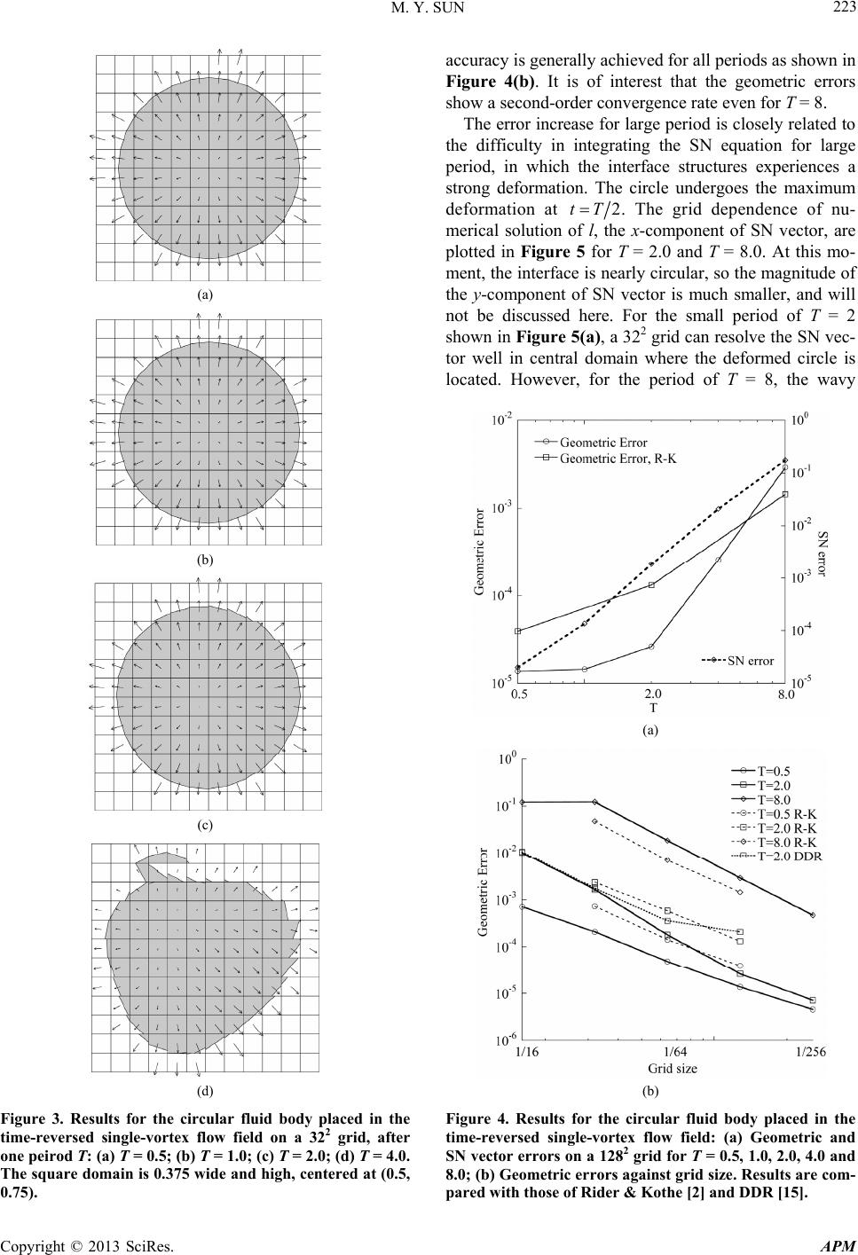

M. Y. SUN 223

(a)

(b)

(c)

(d)

Figure 3. Results for the circular fluid body ed in the

time-reversed single-vortex flow field on a 3 grid, after

one peirod T: (a) T = 0.5; (b) 1.0; (c) T = 2.0; (d) T = 4.0.

plac

T =

The square domain is 0.375 wide and high, centered at (0.5,

0.75).

accuracy is generally achieved for all periods as shown in

Figure 4(b). It is of interest that the geometric errors

show a second-order convergence rate even for T = 8.

The error increase for large period is closely related to

the difficulty in integrating the SN equation for large

period, in which the interface structures experiences a

strong deformation. The circle undergoes the maximum

deformation at 2tT



. The grid dependence of nu-

merical solution of l, the x-component of SN vector, are

plotted in Figure 5 for T = 2.0 and T = 8.0. At this mo-

ment, the interface is nearly circular, so the magnitude of

the y-component of SN vector is much smaller, and will

not be discussed here. For the small period of T = 2

shown in Figure 5(a), a 322 grid can resolve the SN vec-

tor well in central domain where the deformed circle is

located. However, for the period of T = 8, the wavy

(a)

(b)

Figure 4. Results for the circular fluid body placed in the

time-reversed single-vortex flow field: (a) Geometric and

SN vector errors on a 1282 grid for T = 0.5, 1.0, 2.0, 4.0 and

8.0; (b) Geometric errors agt grid size. Results are com- ains

pared with those of Rider & Kothe [2] and DDR [15].

M. Y. SUN

224

othods

Table 2. Convergence of the present method that couples the multidimensional advection algorithm with the SN vector equa-

tion in the reversed single-vortex test. A few published resultstained using various advection and reconstruction meb

are compared.

Mesh SN vector Youngs Puckett Quadratic

∆x Present 15] H & F [17] [9] R & K [2] [9] DDR [ EMPAEMPAEL-LE [8]

1/8 4.−2 4.−2 70 × 1074 × 10- - - - -

1/16 −2−2

−3−32.49 × 10−3 2.29 × 10−3 2.36 × 10−3 2.14 × 10−3 1.88 × 10−3

−4−4−4−4−4−4−4

1/128 −3−4−4−4−4−4−5

1.02 × 10 1.06 × 10 - - - - -

1/32 1.65 × 10 1.76 × 10

1/64 1.80 × 10 3.58 × 10 7.06 × 10 6.72 × 10 5.85 × 10 5.39 × 10 4.42 × 10

2.61 × 10 2.08 × 10 2.23 × 10 2.24 × 10 1.31 × 10 1.29 × 10 9.36 × 10

(a)

Figure 5. Numerical solution-component of SN vecl)

along y = 0.5 at t = T/2: (a) T (b) T = 8.

at difficulty

e solution to converge. The numerical error of the

affetionent

The geometric errors of the PLIC/SN method are com-

ns as low

(b)

remain andct the solu at last mom.

of x

= 2;tor (

structure of the SN vector imposes a gre for

SN th

vector introduced in the stage of large deformation may

pared with other results in literature in Table 2. The pre-

sent results show an improved accuracy for all grids. The

grid convergence is achieved for grid resolutio

18x



. Compared with the DDR advection, the geo-

metric errors at high resolution grids



164,1128x

have been greatly reduced. For 1 128x , the geomet-

rical error





2.61 10

 is only a bit larger than that in

the ion test. To what we know, this accuracy has

never been reported before.

4. Concluding Remarks

It has been shown shown that the equation of allow us to

implicitly track a subgrid

translat

particle [15] when coupled

is work confirms that the

with the multidimensional

d (VOF)

Method for the Dynamics of Free Boundaries,” Journal

of Computationa, 1981, pp. 201-

225. doi:10.10 -5

with the PLIC-VOF method. Th

equation of SN vector coupled

advection algorithm improves the accuracy not only on

low resolution grids but also on high resolution grids in

the vortical flows with a low period. The geometric error

obtained is much lower than those reported in literature.

The PLIC/SN method generally improves the accuracy

in the calculation of SN vector, especially at low grid

resolution. It can resolve a particle with less cells, or re-

solve more particles/bubbles with a given grid. In the

rect simulation of interfacial phenomena with a large

amount of particles/bubbles, such as defragmentation,

cavitation, it is expected that the PLIC/SN can resolve

interfacial structure with one order of magnitude less grid

cells for achieving the same interface resolution.

REFERENCES

[1] C. W. Hirt and B. D. Nichols, “Volume of Flui

l Physics, Vol. 39, No. 1

16/0021-9991(81)90145

[2] W. J. Rider and D. B. Kothe, “Reconstructing Volume

Tracking,” Journal of Computational Physics, Vol. 141,

No. 2, 1998, pp. 112-152. doi:10.1006/jcph.1998.5906

M. Y. SUN 225

[3] R. Scardovelli and S. Zaleski, “Direct Numerical Simula-

tion of Free-Surface and Interfacial Flow,” Annual Re-

view of Fluid Mechanics, Vol. 31, 1999, pp. 567-603.

doi:10.1146/annurev.fluid.31.1.567

[4] W. F. Noh and P. Woodward, “SLIC (Simple Line Inter-

face Calculation),” In: A. I. van der Vooren and P. J.

Zandbergen, Eds., Lecture Notes in Physics, Springer,

New York, 1976, p. 330.

[5] M. Rudman, “Volume-Tracking Methods for Interfacial

Flow Calculations,” International Journal for Numerical

Methods in Fluids, Vol. 24, No. 7, 1997, pp. 671-691.

doi:10.1002/(SICI)1097-0363(19970415)24:7<671::AID-

FLD508>3.0.CO;2-9

[6] D. L. Youngs, “An Interface Tracking Method for a 3D

Eulerian Hydrodynamics Code,” Technical Report 44/92/

35, AWRE, 1984.

[7] E. G. Puckett, “A Volume of Fluid Interface Tracking

Algorithm with Applications to Computing Shock Wave

S. Zaleski, “Interface Reconstruction

Rarefraction,” Proceedings of the 4th International Sym-

posium on Computational Fluid Dynamics, 1991.

[8] R. Scardovelli and

with Least-Square Fit and Split Eulerian-Lagrangian Ad-

vection,” International Journal for Numerical Methods in

Fluids, Vol. 41, No. 3, 2003, pp. 251-274.

doi:10.1002/fld.431

[9] J. López, J. Hernández, P. Gómez and F. Faura, “A Vol-

ume of Fluid Method Based on Multidimensional Advec-

tion and Spline Interface Reconstruction,” Journal of

Computational Physics, Vol. 195, No. 2, 2004, pp. 718-

742. doi:10.1016/j.jcp.2003.10.030

[10] J. E. Pilliod Jr. and E. G. Puckett, “Second-Order Accu-

rate Volume-of-Fluid Algorithms for Tracking Material

Interfaces,” Journal of Computational Physics, Vol. 199,

No. 2, 2004, pp. 465-502. doi:10.1016/j.jcp.2003.12.023

[11] M. M. Francois and B. K. Swartz, “Interface Curvature

via Volume Fractions, Heights, and Mean Values on

Nonuniform Rectangular Grids,” Journal of Computa-

tional Physics, Vol. 229, No. 3, 2010, pp. 527-540.

doi:10.1016/j.jcp.2009.10.022

[12] M. Sussman and E. G. Puckett, “A Coupled Level Set and

Volume-of-Fluid Method for Computing 3D and

symmetric Incompressible Two

Axi-

-Phase Flows,” Journal of

Computational Physics, Vol. 162, No. 2, 2000, pp. 301-

337. doi:10.1006/jcph.2000.6537

[13] M. Raessi, J. Mostaghimi and M. Bussmann, “Advecting

Normal Vectors: A New Method for Calculating Interface

Normals and Curvatures When Modeling Two-Phase

Flows,” Journal of Computational Physics, Vol. 226, No.

1, 2007, pp. 774-794. doi:10.1016/j.jcp.2007.04.023

[14] D. J. E. Harvie and D. F. Fletcher, “A New Volume of

Fluid Advection Algorithm: The Defined Donating Re-

gion Scheme,” International Journal for Numerical Me-

thods in Fluids, Vol. 35, No. 2, 2001, pp. 151-172.

doi:10.1002/1097-0363(20010130)35:2<151::AID-FLD8

7>3.0.CO;2-4

[15] M. Sun, “Volume Tracking of Subgrid Particles,” Inter-

national Journal for Numerical Methods in Fluids, Vol.

66, No. 12, 201

1, pp. 1530-1554. doi:10.1002/fld.2331

[16] D. Igra and M. Sun, “Shock-Water Column Interaction,

from Initial Impact to Fragmentation Onset,” AIAA Jour-

nal, Vol. 48, No. 12, 2010, pp. 2763-2771.

doi:10.2514/1.44901

[17] D. J. E. Harvie and D. F. Fletcher, “A New Volume of

Fluid Advection Algorithm: The Stream Sch

nal of Computational eme,” Jour-

Physics, Vol. 162, No. 1, 2000, pp.

1-32. doi:10.1006/jcph.2000.6510
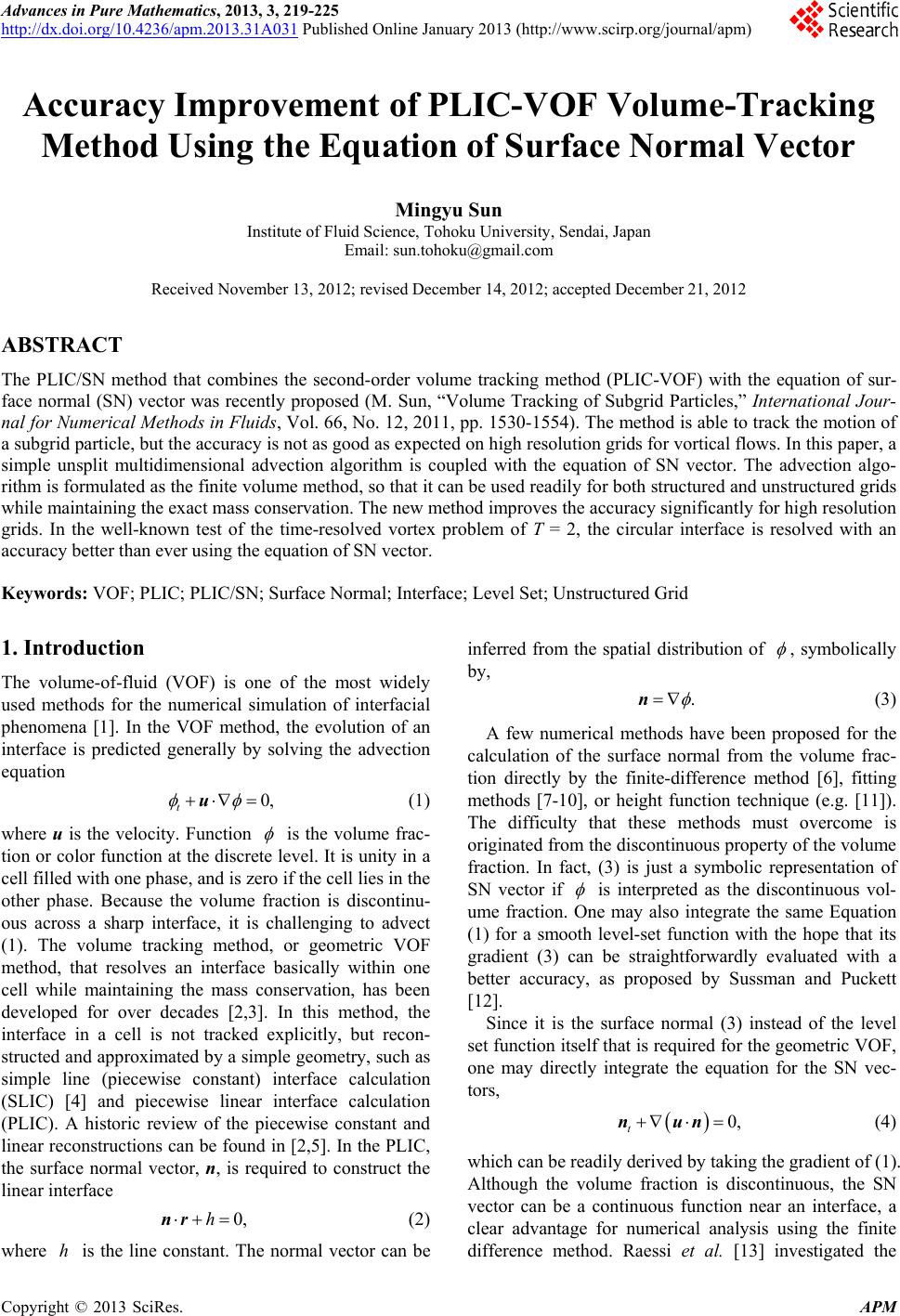