 Vol.2, No.9, 929-947 (2010) Natural Science http://dx.doi.org/10.4236/ns.2010.29115 Copyright © 2010 SciRes. OPEN ACCESS Baryon wave functions and free neutron decay in the scalar strong interaction hadron theory (SSI) F. C. Hoh Dragarbrunnsg. 55C, Uppsala, Sweden; hoh@telia.com Received 16 June 2010; revised 19 July 2010; accepted 25 July 2010. ABSTRACT From the equations of motion for baryons in the scalar strong interaction hadron theory (SSI), two coupled third order radial wave equations for baryon doublets have been derived and published in 1994. These equations are solved numerically here, using quark masses obtained from meson spectra and the masses of the neutron, 0 and 0 as input. Confined wave functions dependent upon the quark-diquark distance as well as the values of the four inte- gration constants entering the quark-diquark interaction potential are found approximately. These approximative, zeroth order results are employed in a first order perturbational treat- ment of the equations of motion for baryons in SSI for free neutron decay. The predicted mag- nitude of neutron’s half life agrees with data. If the only free parameter is adjusted to produce the known A asymmetry coefficient, the pre- dicted B asymmetry agrees well with data and vice versa. It is pointed out that angular mo- mentum is not conserved in free neutron decay and that the weak coupling constant is detached from the much stronger fine structure constant of electromagnetic coupling. Keywords: Scalar Strong Interaction; Baryon Radial Wave Functions; Free Neutron Decay 1. INTRODUCTION This paper consists of two parts. In Part 2, the equations of motion of ground state dou- blet baryons in the scalar strong interaction hadron the- ory (SSI) derived earlier are solved numerically to yield approximate baryon wave functions and quark-diquark interaction potential. In Part 3, these results are employed in free neutron decay to obtain decay time and the A and B asymmetry coefficients. Nonconservation of angular moemntum and detachment of weak and electromagnetic couplings are pointed out. 2. BARYON WAVE FUNCTIONS 2.1. Conversion to Six First Order Equations Although the equations of motion for mesons [1] and for baryons [2] in the scalar strong interaction hadron theory (SSI) were both published in the early 1990’s, subse- quent work took place wholly in the meson sector. This due to that the meson equations can be decomposed into second order differential equations Eqs.6.7-8 of [1] or Eqs.3.2.3-4 of [3] which have analytical solutions in the rest frame providing the zeroth order background upon which higher order perturbational problems can be built and treated. Much success and new insights about mes- ons have been achieved, as are seen in Chapters 4-8 in [3]. Of current interest is that no Higgs boson is nee- ded to generate the mass of the gauge boson [4]. The linear Dalitz plot slope parameters in kaon decaying into three pions [5] and electromagnetic and strong decays of some vector mesons [6] have been treated. The epistemologi- cal foundation of SSI is given in the recent [7]. On the other hand, the two coupled third order radial equations for baryon doublets Eq.A20 cannot be decou- pled and reduced to lower order equations. They are eve- ntually reduced to the six first order equations Eq.1 be- low which have to be solved numerically. Further, the interquark potential Eq.A15 contains four unknown in- tegration constants that enter Eq.1. Very lengthy work has been spent in finding these constants and solving Eq.1 below by computer. This is the reason that the baryon re- sults to be presented below come so many years later. Such numerical computations have been carried out and the four integration constants in Eq.A15 and Eq.1 are obtained together with the radial wave functions. The coupled third order equations Eq.A20 cannot be solved analytically and have to be treated numerically.  F. C. Hoh / Natural Science 2 (2010) 929-947 Copyright © 2010 SciRes. OPEN ACCESS 930 The standard procedure is to convert them into a first sy- stem according to Eq.10.7.5 of [3] after putting the or- bital angular momentum L = 0 there (see Eq.1), In arriving at Eq.1, Eq.A15 has been used. E0 is the neutron mass, Mb 3 is the quark mass term defined in Eq.A4 and the four db constants are integration constants in the solution to the homogenized Eq.A14 b(r) = 0 and are independent of flavor, i.e., baryon species, as was pointed out below Eq.10.1.6 of [3]. These four db constants can therefore not be fixed by using four baryon masses as input. The procedure ado- pted is as follows. The quarks masses in Eq.A4 are mu 0.6592, md mu 0.00215 and ms 0.7431 in units of Gev taken from Table 1 of [8] or Table 5.2 of [3] obtain- ned from meson spectra. Three known baryon masses are E0 0.9397, 1.1926 and 1.3148 Gev for neutron, 0 and 0, respectively [9]. These are inserted into Eq.1 and the four db’s are varied over suitable ranges such that the solutions satisfy the boundary condition at r or converge there. Near the origin r 0, the baryon radial wave func- tions can be expanded in power series in r according to Eq.10.7.6 of [3], 00 , rbrgrarf oo (2) where satisfy the indicial equation Eq.10.7.4 of [3] and is related to + in Eq.4 below. a and b are constants satisfying the recursion formula Eq.10.7.7 of [3]. At large r, Eq.10.2.7a of [3] gives 3 5 3 1 2 00 5 3 expconstant rd rfrg b (3) The presence of r1/3 is incompatible with the power series Eq.2 and Eq.1 has to be solved numerically. Equivalent to Eq.2 is the expansion around the regular singular point r = 0 in Eq.1, 0, 1,2,....6 wr wrrwr (4) where + are given by Eq.10.2.8a of [3]. The three cases with possible + 0 are excluded because they lead to diverging w (r = 0). The remaining cases yield 0,1,0 100400 ww (5) 1101401 ,0,1 www (6) 0,,2 1022402 www (7) where the amplitude in Eq.5 has been normalized to unity. w(1) and w(2) are amplitudes for the remaining two solutions. The general solution near r 0 reads rwrwrwrw 210 (8) Substituting this into Eq.1 , which is now solved as an initial value problem with initial conditions Eqs.5-7. 2.2. Numerical Solution and Results The six unknown parameters db, d b0, d b1, d b2, w(1), and w(2) are adjusted so that the six boundary conditions w (r ) 0 for a given Mb 3 and the associated baryon mass E0. The calculations are done via a Fortran progr- am employing Runge-Kutta integration subroutine on computers of the Department of Information Technology at Uppsala University. In the paramater range of interest, it was found that integration of Eq.1 and summation of the power series Eq.2 give the nearly the same results for r 7-8 Gev1. Beyond this value, Eq.2 become unre- liable due to accumulated computational errors. Simi- larly, Eq.1 leads often to diverging solutions at r 7-12. This is because that Eq.3 without the minus sign in the exponent is also a solution which tends to overshadow Eq.3 due to accumulated errors and takes over at large r. Near the origin r 0 and at large r, the potential in Eq.1 is dominated by the db/r and db2r2, respectively, and the flavor dependent quark mass term Mb 3 there can be dropped. The solutions f0(r) and g0(r) in these r regions are independent of the baryon flavor. Thus, db and db2 are flavor independent constants on par with the corresp- onding meson sector’s dm and dm0 which are independent of flavor according to Subsection 4.4 of [3]. The small r region is very small and the large r region determines the asymtotic behavior of f0(r) and g0(r). r wr E r w E ww Erdrd r dM E r d w r w E ww rdrd r dM E r d w r wr E r wr E w r w r w r w r w r w r w r w r w r w rgrwrfrw bbbbb bbbbb 1 4 2 2 8 2 8 1 4 2 2 4 , , , , 6 2 0 5 0 320 4 2 3 1 2 0 3 3 0 1 6 0 65 4 2 3 1 2 0 3 3 0 43 2 0 2 2 0 1 3 65543221 0401 (1) 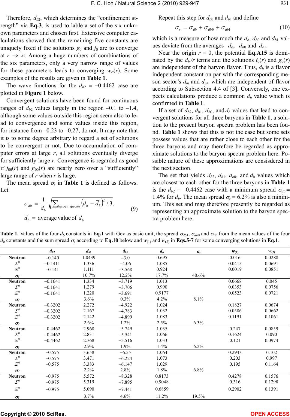 F. C. Hoh / Natural Science 2 (2010) 929-947 Copyright © 2010 SciRes. OPEN ACCESS 931 931 Therefore, db2, which determines the “confinement st- rength” via Eq.3, is used to lable a set of the six unkn- own parameters and chosen first. Extensive computer ca- lculations showed that the remaining five constants are uniquely fixed if the solutions g0 and f0 are to converge at r . Among a huge numbers of combinations of the six parameters, only a very narrow range of values for these parameters leads to converging w (r). Some examples of the results are given in Table 1. The wave functions for the db2 0.4462 case are plotted in Figure 1 below. Convergent solutions have been found for continuous ranges of d b2 values largely in the region –0.1 to –1.4, although some values outside this region seem also to le- ad to convergence and some values inside this region, for instance from –0.23 to –0.27, do not. It may note that it is to some degree arbitrary to regard a set of solutions to be convergent or not. Due to accumulation of com- puter errors at large r, all solutions eventually diverge for sufficiently large r. Convergence is regarded as good if f00(r) and g00(r) are nearly zero over a “sufficiently” large range of r when r is large. The mean spread s in Table 1 is defined as follows. Let bb bb b db dd dd d of valueaverage ,3/ 1 speciesbaroyn 2 (9) Repeat this step for db0 and db1 and define 10 dbdbdbs (10) which is a measure of how much the db, db0 and db1 val- ues deviate from the averages db, db0 anddb1. Near the origin r = 0, the potential Eq.A15 is domi- nated by the db /r terms and the solutions f0(r) and g0(r) are independent of the baryon flavor. Thus, db is a flavor independent constant on par with the corresponding me- son sector’s dm and dm0 which are independent of flavor according to Subsection 4.4 of [3]. Conversely, one ex- pects calculations produce a common db value which is confirmed in Table 1. If a set of db2, db1, db0, and db values that lead to con- vergent solutions for all three baryons in Table 1, a solu- tion to the present baryon spectra problem has been fou- nd. Table 1 shows that this is not the case but some sets possess values that are rather close to each other for the three baryons and may therefore be regarded as appro- ximate solutions to the baryon spectra problem here. Po- ssible nature of these approximations are consisdered in the next section. The set that yields db2, db1, db0, and db values which are closest to each other for the three baryons in Table 1 is the db2 = 0.4462 case with a minimum spread db 1.4% for db. The mean spread s 6.2% is also a minim- um. This set and may therefore presently be regarded as representing an approximate solution to the baryon spec- tra problem here. Table 1. Values of the four db constants in Eq.1 with Gev as basic unit, the spread db1, db0 and db from the mean values of the four db constants and the sum spread s according to Eq.10 below and w(1) and w(2) in Eqs.5-7 for some converging solutions in Eq.1. db2 db1 db0 db s w(1) w(2) Neutron 0.140 1.0439 3.0 0.695 0.016 0.0288 0 0.1411 1.336 4.06 1.085 0.0415 0.0691 0 0.141 1.111 3.568 0.924 0.0019 0.0851 d 10.7% 12.2% 17.7% 40.6% Neutron 0.1641 1.334 3.719 1.013 0.0668 0.045 0 0.1641 1.279 3.706 0.990 0.0353 0.0756 0 0.1641 1.220 3.691 0.9177 0.0523 0.0721 d 3.6% 0.3% 4.2% 8.1% Neutron 0.3202 2.272 4.922 1.024 0.1827 0.0674 0 0.3202 2.167 4.783 1.032 0.0586 0.0662 0 0.3202 2.142 4.899 1.083 0.1191 0.1061 d 2.6% 1.2% 2.5% 6.3% Neutron 0.4462 2.968 5.749 1.035 0.247 0.0859 0 0.4462 2.831 5.541 1.066 0.1624 0.090 0 0.4462 2.768 5.516 1.033 0.121 0.0974 d 2.9% 1.9% 1.4% 6.2% Neutron 0.575 3.658 6.55 1.064 0.2943 0.102 0 0.575 3.471 6.224 1.073 0.203 0.997 0 0.575 3.383 6.147 1.029 0.195 0.1164 d 2.2% 2.8% 1.8% 6.8% Neutron 0.975 5.572 8.328 0.8173 0.4278 0.1576 0 0.975 5.319 7.895 0.9048 0.316 0.1298 0 0.975 5.090 7.441 0.6859 0.2902 0.1391 d 3.7% 4.6% 11.2% 19.5% 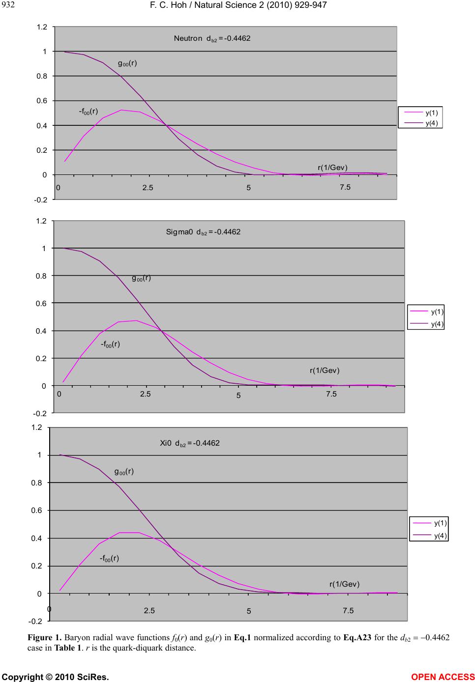 F. C. Hoh / Natural Science 2 (2010) 929-947 Copyright © 2010 SciRes. OPEN ACCESS 932 0.2 0 0.2 0.4 0.6 0.8 1 1.2 y(1) y(4) Neutron d b2 = -0.4462 g 00 (r) -f 00 (r) r(1/Gev) 05 2.5 7.5 -0.2 0 0.2 0.4 0.6 0.8 1 1.2 y(1) y(4) g 00 (r) -f 00 (r) 05 r(1/Gev) Sigma0 d b2 = -0.4462 2.5 7.5 -0.2 0 0.2 0.4 0.6 0.8 1 1.2 y(1 ) y(4 ) g 00 (r) -f 00 (r) 0 r(1/Gev) 5 Xi0 d b2 = -0.4462 2.5 7.5 Figure 1. Baryon radial wave functions f0(r) and g0(r) in Eq.1 normalized according to Eq.A23 for the db2 0.4462 case in Table 1. r is the quark-diquark distance. 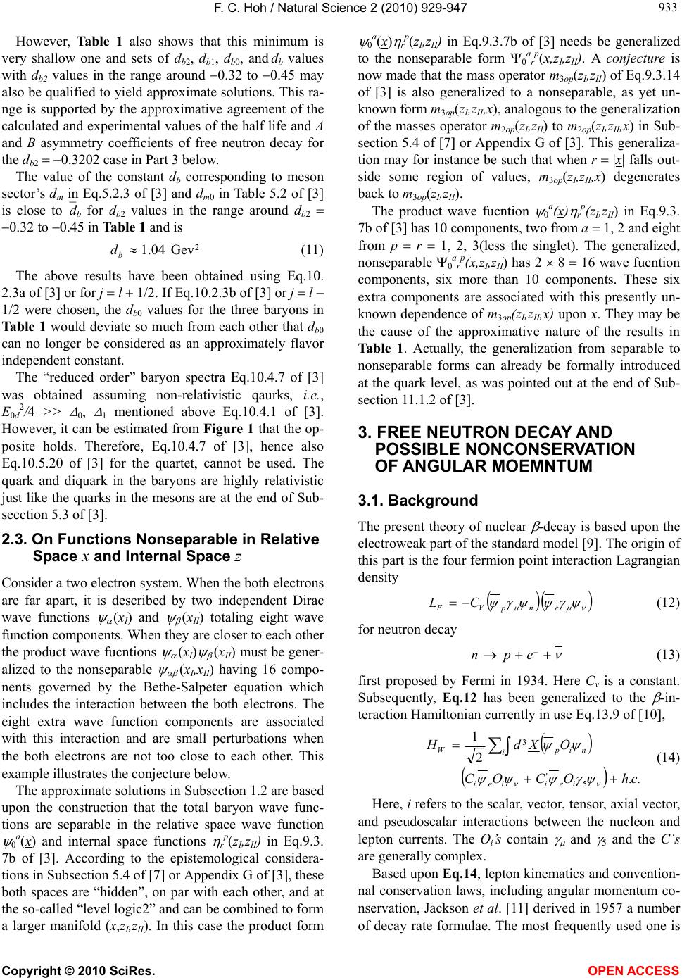 F. C. Hoh / Natural Science 2 (2010) 929-947 Copyright © 2010 SciRes. OPEN ACCESS 933 933 However, Table 1 also shows that this minimum is very shallow one and sets of db2, db1, db0, and db values with db2 values in the range around 0.32 to 0.45 may also be qualified to yield approximate solutions. This ra- nge is supported by the approximative agreement of the calculated and experimental values of the half life and A and B asymmetry coefficients of free neutron decay for the db2 0.3202 case in Part 3 below. The value of the constant db corresponding to meson sector’s dm in Eq.5.2.3 of [3] and dm0 in Table 5.2 of [3] is close todb for db2 values in the range around db2 0.32 to 0.45 in Table 1 and is 2 Gev04.1 b d (11) The above results have been obtained using Eq.10. 2.3a of [3] or for j l 1/2. If Eq.10.2.3b of [3] or j l 1/2 were chosen, the db0 values for the three baryons in Table 1 would deviate so much from each other that db0 can no longer be considered as an approximately flavor independent constant. The “reduced order” baryon spectra Eq.10.4.7 of [3] was obtained assuming non-relativistic qaurks, i.e. , E0d 2/4 >> 0, 1 mentioned above Eq.10.4.1 of [3]. However, it can be estimated from Figure 1 that the op- posite holds. Therefore, Eq.10.4.7 of [3], hence also Eq.10.5.20 of [3] for the quartet, cannot be used. The quark and diquark in the baryons are highly relativistic just like the quarks in the mesons are at the end of Sub- secction 5.3 of [3]. 2.3. On Functions Nonseparable in Relative Space x and Internal Space z Consider a two electron system. When the both electrons are far apart, it is described by two independent Dirac wave functions (xI) and (xII) totaling eight wave function components. When they are closer to each other the product wave fucntions (xI) (xII) must be gener- alized to the nonseparable (xI,xII) having 16 compo- nents governed by the Bethe-Salpeter equation which includes the interaction between the both electrons. The eight extra wave function components are associated with this interaction and are small perturbations when the both electrons are not too close to each other. This example illustrates the conjecture below. The approximate solutions in Subsection 1.2 are based upon the construction that the total baryon wave func- tions are separable in the relative space wave function 0 a(x) and internal space functions r p(zI,zII) in Eq.9.3. 7b of [3]. According to the epistemological considera- tions in Subsection 5.4 of [7] or Appendix G of [3], these both spaces are “hidden”, on par with each other, and at the so-called “level logic2” and can be combined to form a larger manifold (x,zI,zII). In this case the product form 0 a(x) r p(zI,zII) in Eq.9.3.7b of [3] needs be generalized to the nonseparable form 0 a r p(x,zI,zII). A conjecture is now made that the mass operator m3op(zI,zII) of Eq.9.3.14 of [3] is also generalized to a nonseparable, as yet un- known form m3op(zI,zII,x), analogous to the generalization of the masses operator m2op(zI,zII) to m2op(zI,zII,x) in Sub- section 5.4 of [7] or Appendix G of [3]. This generaliza- tion may for instance be such that when r |x| falls out- side some region of values, m3op(zI,zII,x) degenerates back to m3op(zI,zII). The product wave fucntion 0 a(x) r p(zI,zII) in Eq.9.3. 7b of [3] has 10 components, two from a 1, 2 and eight from p r 1, 2, 3(less the singlet). The generalized, nonseparable 0 a r p(x,zI,zII) has 2 8 16 wave fucntion components, six more than 10 components. These six extra components are associated with this presently un- known dependence of m3op(zI,zII,x) upon x. They may be the cause of the approximative nature of the results in Table 1. Actually, the generalization from separable to nonseparable forms can already be formally introduced at the quark level, as was pointed out at the end of Sub- section 11.1.2 of [3]. 3. FREE NEUTRON DECAY AND POSSIBLE NONCONSERVATION OF ANGULAR MOEMNTUM 3.1. Background The present theory of nuclear -decay is based upon the electroweak part of the standard model [9]. The origin of this part is the four fermion point interaction Lagrangian density enpVF CL (12) for neutron decay epn (13) first proposed by Fermi in 1934. Here Cv is a constant. Subsequently, Eq.12 has been generalized to the -in- teraction Hamiltonian currently in use Eq.13.9 of [10], .. 2 1 5 ' 3 chOCOC OXdH i e ii e i ni p i W (14) Here, i refers to the scalar, vector, tensor, axial vector, and pseudoscalar interactions between the nucleon and lepton currents. The Oi’s contain and 5 and the C´s are generally complex. Based upon Eq.14, lepton kinematics and convention- nal conservation laws, including angular momentum co- nservation, Jackson et al. [11] derived in 1957 a number of decay rate formulae. The most frequently used one is  F. C. Hoh / Natural Science 2 (2010) 929-947 Copyright © 2010 SciRes. OPEN ACCESS 934 ... 1 constant 33 e e e e e e e n n e e npe e E K R EE KK D E K B E K A J J EE KK a EEEEKdKddW (15) in which the final spins have been summed over for a given initial neutron polarization Jn . Here, the K’s de- note momenta, E energy and e the electron polarization. The constants a, A, B, D, R, and depend upon the C´s and the nucleon current consisting of a vector and an axial vector part in the so-called V-A theory. Experi- ments on neutron decay have since then largely been devoted to determine these constants in this nearly 50 year old Eq.15 and related formulae [12]. These have, however, yielded little physical insight into the decay mechanism. The standard Hamiltonian Eq.14 is a phenomenology- ical model, not derivable from any first principles theory. It treats nucleon as a point particle and hence ignores its quark structure. There are in principle 20 real C con- stants in Eq.14, leaving the theory with little predictive power. This hints at a superfluousness of Eq.1 4, which is not invariant under SU(2) gauge transformations. Such an invariance would give rise to an intermediate vector boson W which couples to a left-handed e pair. Therefore, despite its noble origin and general accep- tance, this model Eq.14 does not differ in principle from the large number of recent phenomenological models, constructed for different and narrow application angles, present in a vast body of literature. Angular momentum conservation has not been establ- ished experimentally in free neutron decay. Most of the experiments make use of nuclei and the conclusion is that angular momentum is conserved. But a nucleus poses a highly complex, unsolved many body problem and exp- eriments with it cannot lead to any firm conclusion on angular momentum conservation in free neutron decay. In this part, free neutron decay will be treated using the equations of motion for doublet baryons Eqs.A7-A8 and its development in Chapters 9-11 of [3], incorporating vector gauge fields of Eqs.12-13 of [4] or Subsection 7.1.2 of [3] and new tensor gauge fields. The results obtained, not reachable from Eq.15, include a prediction of the half life of the neutron in approximate agreement with data and a relatively good prediction of the B asymmetry coefficient. 3.2. Introduction of Vector and Tensor Gauge Fields 3.2.1. Action-Like Integrals for Doublet Baryons The starting point is the equation of motion for doublet baryons Eqs.A7-A8. Multiply Eq.A7 from the left by 0a * and Eq.A8 by b * 0 , subtract the resulting expres- sions from their complex conjugates and integrate over xI and xII to obtain .. 2 1 00 3 2 1 0 44' ccMi dxdx i S a abb fhb ba I he I ef IIaIII (16) .. 2 1 0 * 0 3 2 1 * 0 44' ccMi dxdx i S b b bb eck cbIkhI heII b III (17) where * is an extra sign denoting complex conjugate, I / xI and II / xII and their positions have been chan- ged so that the summations over the e and h indices con- form to matrix multiplication convention and that the bo- th I’s appear next to each other to reflect that they oper- ate on the diquark part indicated by the braces. These integrals will not be varied with respect to 0a * and b * 0 in an attempt to reproduce Eqs.A7-A8; han- dling of the last c.c. terms and the necessary boundary conditions will require efforts beyond the scope of this chapter. Nor is such a variation necessary for the present purposes. If the solutions to Eqs.A7-A8 is inserted into Eqs.16-17, we obtain 0,0 ' 0 '' 0 ' SSSS (18) 3.2.2. Non-Minimal Substitution and Tensor Gauge Field The minimal substitution of Eq.12 of [4] or Eq.7.1.4 of [3] led to the introduction of the vector gauge boson field W which is naturally associated with the vector part V of the V-A theory mentioned beneath Eq.15. The axial vector part A is an asymmetrical part of a tensor which can be introduced by the following non-minimal substi- tution (see Eq s.19 -20), fhb bahebahehe I baba I he fbh ba I he I fbh ba I he IXWXgW i XTXWXWg i 42 1 4 (19) eck cbkhcbkhkhIcbcbIkh ekc cbIkhI ekc cbIkhI XWXgW i XTXWXWg i 42 1 4 (20) 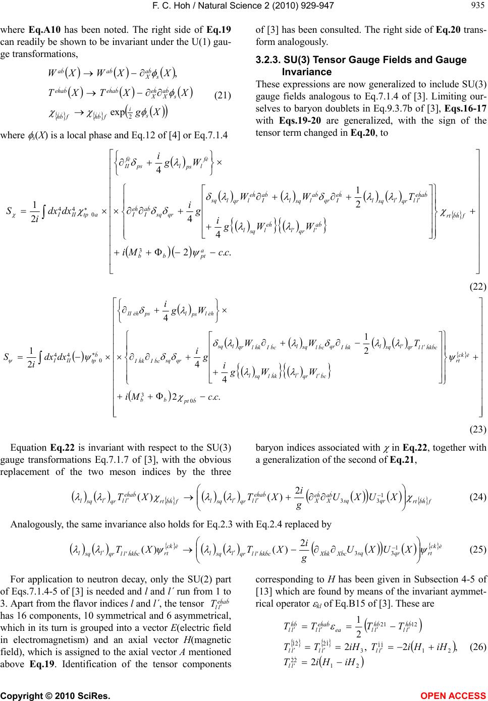 F. C. Hoh / Natural Science 2 (2010) 929-947 Copyright © 2010 SciRes. OPEN ACCESS 935 935 where Eq.A10 has been noted. The right side of Eq.19 can readily be shown to be invariant under the U(1) gau- ge transformations, Xg XXTXT XXWXW s i fbhfbh s ba X he X bahebahe s ba X baba 2 exp , (21) where s(X) is a local phase and Eq.12 of [4] or Eq.7.1.4 of [3] has been consulted. The right side of Eq.20 trans- form analogously. 3.2.3. SU(3) Tensor Gauge Fields and Gauge Invariance These expressions are now generalized to include SU(3) gauge fields analogous to Eq.7.1.4 of [3]. Limiting our- selves to baryon doublets in Eq.9.3.7b of [3], Eqs.16-17 with Eqs.19-20 are generalized, with the sign of the tensor term changed in Eq.20, to .. 2 4 2 1 4 4 2 1 3 0 44 ccMi WWg i TWW g i Wg i dxdx i S a ptbb fhbrt ba l qr l he l sq l bahe ll qr l sq l he Iqr ba l sq l ba I he l qr lsq qrsq ba I he I ef l ps lps ef II atpIII (22) ..2 4 2 1 4 4 2 1 0 3 * 0 44 ccMi WWg i TWW g i Wg i dxdx i S bpt bb eck rt cbl qr l khl sq l cbkhll qr l sq l khI qr cbl sq l cbIkhl qr lsq qrsq cbIkhI hel ps lpsheII b tpIII (23) Equation Eq.22 is invariant with respect to the SU(3) gauge transformations Eq.7.1.7 of [3], with the obvious replacement of the two meson indices by the three baryon indices associated with in Eq.22, together with a generalization of the second of Eq.21, fhbrt qrsq ba X he X bahe ll qr l sq l fhbrt bahe ll qr l sq lXUXU g i XTXT 1 33 2 )()( (24) Analogously, the same invariance also holds for Eq.2.3 with Eq.2.4 replaced by eck rtqrsq cbXkhXcbkhll qr l sq l eck rt cbkhll qr l sq lXUXU g i XTXT 1 33 2 )()( (25) For application to neutron decay, only the SU(2) part of Eqs.7.1.4-5 of [3] is needed and l and l´ run from 1 to 3. Apart from the flavor indices l and l´, the tensor bahe ll T has 16 components, 10 symmetrical and 6 asymmetrical, which in its turn is grouped into a vector E(electric field in electromagnetism) and an axial vector H(magnetic field), which is assigned to the axial vector A mentioned above Eq.19. Identification of the tensor components corresponding to H has been given in Subsection 4-5 of [13] which are found by means of the invariant aymmet- rical operator kl of Eq.B15 of [3]. These are 21 22 21 11 3 1221 1221 2 ,2 ,2 2 1 iHHiT iHHiTiHTT TTTT ll llllll bh ll bh llea bahe ll bh ll (26)  F. C. Hoh / Natural Science 2 (2010) 929-947 Copyright © 2010 SciRes. OPEN ACCESS 936 The remaining 13 components of bahe ll T do not enter here and are put to zero. 3.3. First Order Relations The gauge boson and tensor field in Eqs.22-23 are decay products of the neutron whose wave functions now ac- quire a weak time dependence. Follow Eq.6.4.1 or Eq.7. 3.1 of [3], noting Eq.A10, and let the nucleon wave fun- ctions in Eqs.22-23 take the form ,,exp ,1 exp , 1 0 0 0 01 001 xXXKiiEXx xX a Xa XKiiEXxXaa xX fhbfhb fhb op op fhb opop fhb (27) where E is the energy, K the momentum, a op 1 and aop (1)(X ) is a first order quantity varying slowly with time. Both can be elevated to operators in quantized case, as are described beneath Eq.6.4.2 of [3]. Ordering of these small quantities aop (1)(X), g, W etc is the same as that in Eqs.18-19 of [4] or Eq.7.3.2 of [3]. The subsc- ripts 0, 1 denote zeroth order and first order quantities, respectively. Following the rudimentary quantization procedure of Eqs.23-25 of [4] or Eqs.6.4.12-15 of [3], let the initial and final states be denoted by W W W W p n KETKEWKpf Kni ,,,, ,0 (28) respectively. n, p, W, T denote the neutron, proton, gauge boson, and tensor gauge field, respectively. Further, 100 ,000 ffii iffi (29) Let aop in Eq.27 and its hermetian conjugate aop + be elevated to annihilation and creation operators. Insert Eq.27 into Eq.22 and sandwich the resulting expression between <f| and |i>. There are two types of first order terms: 1) those containing aop (1)(X0 ) and 2) those linear in gW and gT. Carrrying out integration over the time X0, the type 1) terms read iXaafS x E xixdXdS opopfi a n afi 0)1( 0 2 0 43 , 4 (30) in which the c.c. term in Eq.22 contributes equally. Sfi is the decay amplitude and Eq.A6 has been used. For the evaluation of the type 2) terms, the final state f| in Eq.28 will contain the gauge fields, XKiXiEww XKiXiEw WW XW XiWXW W W ba ba W W ba ba ba ba baba 0 0 0 0 21 exp exp 2 (31) XKiXiEtXT iTiTTT W W bahebahe bahebahebahebahe 0 23323113 exp 2 (32) where Eq.12-13 of [4] or Eq.7.1.4-5 of [3] limited to its SU(2) part has been consulted. The initial and final nu- cleon states in Eq.28 will have a laboratory space time dependence of the form given in Eq.27 with subscripts p for proton and n for neutron attached to the variables there. Here, use has been made of Eq.9.3.7b and Eq.9. 3.18a of [3] which gives tp = 31 for proton and rt = 23 for neutron in Eq.22. After summing over the flavor in- dices t, p, s, q, and r and carrying out the integration over X, the type 2) terms become .. .. 4 2 2 24 0 * 0 0 2 2 * 00 4 4 ccxtxi ccxE E xwxd EEEKK g fhbn eabh ef IIap ann n ap nWp Wp (33) where Eq.A6 has been used and EW and KW terms have been neglected because they are small relative to | I,II |/| |. With Eq.26, Eq.32 and Eq.B5 of [3], the 16 t’s in Eq.33 reduce similarly to three for an axial vetor: XKiXiEtXT XKiXiEtXT ttttt tttttttt tttt tttt W W eaea W W bhbh eaea bh baheea bhbh ea bahebh 0 0 12 21 212112 22 11 1122 11 22 2211 2112 1221 exp ,exp ,, 2 1 , 2 1 (34) 3.4. Decay Amplitude The decay amplitude S fi for the function is found by putting Eq.30 to the negative of Eq.33. Letting d3X, the result is  F. C. Hoh / Natural Science 2 (2010) 929-947 Copyright © 2010 SciRes. OPEN ACCESS 937 937 x E xxd ccxtxiccxE E xwxd EEEKK ig S a n a fhbn eabh ef IIapann n ap nWp Wp fi 0 2 0 3 0 * 00 2 2 * 00 3 4 4 .... 4 2 2 24 (35) In an analogous fashion, The decay amplitude Sfi for the function is obtained from Eq.23 and reads x E xxd ccxtxiccxE E xwxd EEEKK ig S a n a ebh n hbad deII a p a nn n a p nWp Wp fi 0 2 * 0 3 0 *00 2 2 *00 3 4 4 .... 4 2 2 24 (36) The starred wave functions in nominators of Eqs.35- 36 represent final states or proton, irrespective the nucl- eon lables; the c.c. terms will turn out to contribute eq- ually and can be dropped together with an overall factor 2 multiplying the right of Eqs.35-36. The wave functi- ons in denoiminators of Eqs.35-3 6 are those of the initial neutron, as f| has been included in Sfi of Eq.30. The proton may have a different m or spin value in Eqs.A16-A19 relative to that pertaining to the initial neutron in Eqs.35-36. There are four combinations which are denoted by FGTGTF m m notation proton neutron 2 1 2 1 2 1 2 1 2 1 2 1 2 1 2 1 (37) As there are two equally correct solutions Eqs.A16- A17 and Eqs.A18-A19, Eq.30 and Eq.33 are to be av- eraged over these two equally probable solutions. The averaging will turn out to not affect Eq.30 so that it can be carried out for Sfi and Sfi of Eqs.35-36 directly to obtain Sfi av and Sfi av. It removes terms of containing f0(r)g0(r) or their derivatives that will appear in Eqs.35- 36 after application of Eqs.A16-A17 or Eqs.A18-A19 and Eq.37. Such terms will for instance differentiate between neutron spin up and spin down decay rates con- tray to the measured A asymmetry coefficient [9]. In- serting Eqs.A16-A17 and Eqs.A18-A19 into Eq.35 and Eq.36 for the four combinations of Eq.37, making use of Eq.A10, summing over the spinor indices, employing Eq.34, and integrating over the angles and in the relative space, one finds that the both averaged decay am- plitudes Sfi av and Sfi av are the same, as may be expected from the symmetry between the part Eq.22 and the part Eq.23; 12 11 22 12 0 000 2 0 4 33 2 1 0 0 1 2 12 22 t t t t I IEiIIENw N KKEEE g i S S S S SS f gnfgndr dr Wp nWp fiF fiGT fiGT fiF avfiavfi (38)  F. C. Hoh / Natural Science 2 (2010) 929-947 Copyright © 2010 SciRes. OPEN ACCESS 938 0 2 00 2 00 0 2 00 2 00 0 2 0 2 0 0 2 0 2 0,,, rfdrrIrgdrrIrfdrrIrgdrrI fgfg (39) where Ndr is given by Eq.A22 and Ig00 and If00. are defi- ned Eq.A23. 3.5. Expressions for Vector and Tensor Gauge Fields 3.5.1. Mass Generation of W Boson Via Virtual 0 In the analogous meson case, the pion beta decay 0e e of [4] or Subsection 7.4.5 of [3], the gauge boson W decay into a pair of leptons. The mass of the W boson comes from the (gW)2 terms in the meson action integral Sm in Eq.11 of [4] via Eq.32 and Eq.35 of [4] or Sm3 in Eq.7.1.8 of [3] via Eq.7.4.4 and Eq.7.4.6b of [3] and is generated by the integral of the |pion wave functions|2 over the relative space x. It can be seen from Eq.7.4.3a and Eq.7.4.4 of [3] that the energy of pion does not enter and can be zero. In this case, the pion is virtual. In the corresponding action-like integrals S and S of Eqs.22-23, there is no such (gW)2 mass term, only terms of the form (gW)(g I,IIW). Therefore, the gauge boson W from neutron decay cannot decay into a pair of leptons via the integrals Eqs. 22-23 for neutrons. The interpretation of this situation is that gauge bos- onW in the neutron case here decays into a pair of lep- tons via a virtual 0 action as has been considered in Subsection 7.6.2 3 of [3] and employed earlier for muon decay in Subsection 7.6.3 4 of [3]. In the pion beta decay, the W is positively charged and decays into a lepton pair via Eqs.44-45 of [4] or Eq.7.4.10 of [3]. In neutron de- cay, the W is negatively charged and WI in Eq.7.4.5 of [3] is replaced by WI + so that Eq.7.4.5 and Eq.7.4.6a [3], neglecting the first three terms there and noting Eq.7.4.10 of [3], are modified to 2 0 22 2 2 1 2 2 1 1 1 3021 2130 22 Gev42.80 , 22 22 22 dx gM g g WS WWiWW iWWWW M W M W L L L L L L L L La bL ba L W ab I W (40) where the gauge boson mass MW is given by Eq.35 and Eq.41 of [4] or Eq.7.4.6b and Eq.7.4.9 of [3], x0 is the relative time between the quarks in 0 and a large nor- malization volume of the 0. 3.5.2. Variation of the Total Action for Neutron Decay Having found an expression for w0 in Eq.38 from Eq.40 via Eq.31, expressions for the other unknowns tab there will be obtained in this and the next paragraph. The vec- tor gauge boson fields Eq.40 was found by varying the total action Eq.7.1.1 of [3], after removing its last term, or Eq.5 of [4] with respect to W in Subsection 7.4.2 of [3] or Eqs.30-32 of [4]. For neutron decay, the meson action Sm3 in Eq.7.1.1 of [3] is to be replaced by the cor- responding baryons actions Eqs.22-23, S S , and the vector gauge boson action SGB be replaced by a gauge boson-tensor field action SGBT. Equation Eq.5 of [4] or Eq.7.1.1 of [3] is here replaced by LmLavavbGBTTn SSSSSS (41) Here, the lepton actions SL + SLm are the same as those in Eqs.8-10 of [4] or Eqs.7.1.16-17 of [3]. b is a dim- ensionless proportional constant that, for instance, signi- fies that the action-like baryon integrals S and S differ basically from the meson action Sm in Eq.11 of [4] or Sm3 in Eq.7.1.8 of [3] in that the normalization of the wave function amplitudes are different. S av(S av) denotes that S (S ) has been averaged over the both equally pro- bable solutions Eqs.A16-A17 and Eqs.A18-A19 for the baryon wave functions that enter it, just like that Sfi and Sfi of Eqs.35-36 have been averaged to Sfi av and Sfi av in Eq.38. The sign in Eq.41 is chosen because Eq.41 will lead to an expression for tab in Eq.38; if this sign is replaced by , the needed Eq.42 below will vanish. Further, this sign will remove terms linear in gW, as is implied by Sfi av Sfi av 0 from Eq.38. This will cause S av S av in Eq.41 to possess (gW)2 terms, apart from the tab terms, to that order and render it to have an extremum when solutions near the correct ones are inserted into S av S av. Unlike SGB in Eqs.6-7 of [4] or Eq.7.1.2 of [3], SGBT in Eq.41 is unknown. If the tensor gauge field is to have an equation of motion like that for the gauge boson Eqs.34- 35 of [4] or Eq.7.4.6 of [3], SGBT is expected to contain terms of the form ( XW)( XT). Physical existence and interpretation of the tensor gauge field are not known and will be left to eventual future work. For the present purpose, it is sufficient to obtain an expression for tab from Eq.41 for use in Eq.38. Follow the steps of Eqs.30-33 of [4] or Subsection 7.4.2 of [3] and vary Eq.41 with respect to ba W . The unknown S GBT is expected to give rise to en- ergy-momentum terms of the form ( X 2T) corresponding to the first terms on the left of Eq.34 of [4] or Eq.7.4.6a of [3], which have been neglected because they are much smaller than the gauge boson mass term that follows them. Similarly, the obtained ( X 2T) terms can also be  F. C. Hoh / Natural Science 2 (2010) 929-947 Copyright © 2010 SciRes. OPEN ACCESS 939 939 dropped on the same ground so the exact but unknown form of SGBT is of no concern here. Variation of the SL + SLm terms in Eq.41 with respect to ba W is analogous to that given by Eq. 33 of [4] or Eq.7.4.5 of [3] and leads to Eq.40. 3.5.3. Expressions for Tensor and Vector Gauge Fields Variation of S avS av in Eq.41 with respect to ba W is limited to terms of order g2. When evaluating the aver- age S av(S av) using Eqs.A16-A17 and Eqs.A18- A19, it is practically sufficient to use one of them, for instance Eqs.A16-A17 for S (S ) of Eqs.22-23, and drop the f0(r)g0(r) terms, as was mentioned beneath Eq.37. In the evaluation of Eqs.22-23, use is made of Eq.27, Eq.A6 and Eq.A10. When summing over the flavor in- dices t, p, s, q, and r, tp = 32 and rt = 23 for neutron and Eqs.31-32 are employed. Carrying out the angular inte- grations, one finds 3021 2130 UUiUU iUUUU U W SS ab ba avavb (42) 2 2 1 1 3000 2 0 24 1 1 7 3 1 96 L L L L fgn b g XWIIE g U (43) 2 2 1 1 12 000 2 0000 2 3 24 1 1 24 1 1 3 3 1 96 L L L L fg b fgn b g XTII g i WIIE g U (44) 2 1 00 0 11 0 2 21 24 3 32 24 L L fg f b g II I XT g iiUU (45) 0 01 2 0 00 22 0 2 21 , 24 32 3 24 dx g I II XT g iiUU L L f fg b (46) where the upper and lower rows in the U´s refer to neu- tron spin up m 1/2 and spin down m 1/2, respec- tively, in Eqs.A16-A19. Further, Eq.42 has been equated to the negative of Eq.40 as is prescribed in Eq.41. Note that U0 in Eq.43 does not contain W0, which however enters Eq.4 0 and stems from the virtual 0 action in Eq.7.4.4 of [3]. Comparing the X dependence of W’s and T’s and the ’s in Eqs.43-46 via Eq.31, Eq.34 and Eq.7.4.19 of [3], replacing L and L there e and , we find KKKEEE eW eW , (47) Removing the X dependence in Eqs.43-46 and obser- ving Eq.31 and Eq.34, we obtain 1 1 3 96 7 24 1 0 300 2 2 1 1 2 wIIE uuuu g M bfgn L L L L e W (48) 1 1 3 4 3 24 24 0 00 00 2 2 1 1 00 2 12 w II II Ei uuuu g IIM it b fg fg n L L L L e fgW (49) 1 2 2 0 00 22 2 1 2 00 0 11 24 24 32 3 , 24 24 3 32 L L e W f fg b L L e W fg f b uu g M i I II t uu g M i II I t (50) The w´s in Eq.31 are similarly found from Eq.40 and read 2 2 1 1 2 3 2 2 1 1 2 0 22 1 , 22 1 L L L L e W L L L L e W uuuu g M w uuuu g M w (51) 3.5.4. Decay Amplitude as Function of Lepton Wave Functions Eqs.48-51 can now be inserted into Eq.38. Here, it is noted that the neutron spin is up or m 1/2 for the upper two amplitudes corresponding to the upper case in Eqs.48-50 and down or m 1/2 for the lower two am- plitudes corresponding to the lower case in Eqs. 48-50. Thus, the w0 in the third component of a triplet Eq.44 and Eq.49 become a singlet to be combined to the w0 in Eq.51. Analogously, the singlet Eq.48, when inserted into Eq.38 becomes the third component of a triplet to be combined with Eq.49. Effectively, the 7 W3 in Eq.43 and 3 W0 in Eq.44 change place after insertion into Eq.38. The two terms are not the dominating ones but will lead to the two c’s (< 0.4 or so) in Eq.56 below. The resulting decay amplitude, noting Eq.47 and Eq.39, reads  F. C. Hoh / Natural Science 2 (2010) 929-947 Copyright © 2010 SciRes. OPEN ACCESS 940 2 2 1 1 2 1 1 2 2 2 1 1 30 30 4 2 2 00 000 000 00 1 21 8 L L L L L L L L L L L L FF mGT pGT FF dr ep nep e W fiF fiGT fiGT fiF fi uuuu uu uu uuuu bb b b bb N KKKEEEE M g i S S S S S (52) 0 00 2 001 1 2 F fgndrFF c IIENbb (53) 3 0000 2 00 33 1 3 8 F fgg fg b n FFc IIa II E bb (54) 3 3 16 00 2 00 fgg fg b n GTmGTpGT IIa II E bbb (55) 3 48 7 ,3 16 1 0000 2 3 0000 2 0 fggnF fggbnF IIaEc IIaEc (56) Because b in Eq.41 can be incorporated into the wa- ve functions and , it can be absorbed into the normal- ization condition Eq.10.3.13 of [3] by chosing a different normalization constant or equivalently a different nor- malized amplitude ag given by Eq.A23. 3.6. Decay Rate and Asymmetry Coefficients A and B 3.6.1. Decay Rate As in Eq.7.5.1 of [3], the decay rate is states final 2 dfi TS (57) where Td is a long decay time. The subscript “final sta- tes” refers to four final lepton spin states and all possible momenta of the proton, electron and antineutrino, like that in Eq.7.5.2 of [3]. The decay rates are spinse spins2 2 333 9 1 2 fiGT fiF d ep e GT F S S T KdKdKd (58) The square of Sfi contains squares of the functions in Eq.52, which are “linearized” by Eq.7.5.6 of [3] type of formula. Following the common approach, integration over the recoil momenta Kp in Eq.58 is carried out first. By Eq.47, this gives Kp K Ke, where the superscript () has been dropped. Introduce , ,,321 kkkKK eee eeeeee n KK iKiKKK kiikkk cos ,expsin cos,expsin 3 21 321 (59) These and Eq.52 are inserted into the decay rate ex- pression Eq.58 to produce GT F e e nepee drW GT F I I E m EEEEKdKKdK NM g1 8192 22 245 4 (60) spinse spins sinsin GT F eee GT F i i dddd I I (61) FFFF Fiiiii spinse spins (62) GTGTGTGT GT iiiii spinse spins (63) where the both arrows denote the spin directions, separated by the commas in Eq.7.4.19 of [3], of the electron and the antineutrino and 2 330 3 30 11 k mE K bbk mE K bbi ee e FF ee e FF F  F. C. Hoh / Natural Science 2 (2010) 929-947 Copyright © 2010 SciRes. OPEN ACCESS 941 941 2 303 3 30 11 k mE K bbk mE K bbi ee e FF ee e FF F 2 330 3 30 2 303 3 30 11 11 k mE K bbk mE K bbi k mE K bbk mE K bbi ee e FF ee e FF F ee e FF ee e FF F (64) 2 3 2 3 2 2 3 3 1,1 ,11 k mE K bik mE K bi k mE K bik mE K bi ee e mGT GT ee e pGT GT ee e mGT GT ee e pGT GT 2 3 3 2 2 3 2 3 11, 1,1 k mE K bik mE K bi k mE K bik mE K bi ee e mGT GT ee e pGT GT ee e mGT GT ee e pGT GT (65) Let Mev2933.1 pnpnm mmEE (66) Eq.61 can now be evaluated using Eqs.64-65 and Eq.59. Carrying out the angular integrations, it is found that the cross terms in Eq.64 drop out and one finds ee e GT FF GT F mE E b bb I I 16 22 42 23 20 2 (67) which is independent of the antineutrino energy E = |K |. Carrying out the K integration in Eq.60 using Eq.66, one gets GT F em GT F nep I I E I I EEEEKdK 2 2 (68) where 0 K Ee. Inserting Eqs.67-68 into Eq.60, changing the variable dKeKe to dEeEe and noting Eqs. 53-55 leads to 2 2 3 2 0 24 4 3 22 1 128 1 GT FF eFe drW GT F GT F b bb EPdE NM g (69) 2 22 emeeeeF EEmEEP (70) where me Ee me and PF (Ee) is the conventional Fermi electron energy spectrum. The half life of the neutron to be compared to the kn- own exp = 885.7 sec. is 2log 1 2 2log GTF th h (71) where h is the Planck constant. 3.6.2. Asymmetry Coefficients A and B The asymmetry coefficients A and B are obtained from Eq.61, just like Eq.67 , but without carrying out integra- tion over and e, respectively. One finds, FGTmGTFFFGTpGTFF mGTFFFGTpGTFFFGTFGT e e e ee e FGT FGT ee GTF GTF bbbbAbbbbA bbbbbbbbb E K A mE E b b d II II 2 30 2 30 223 20 22 3 20 2 44 2222 cos1 8 4sin (72) The antineutrino moves in the opposite direction rela- tive to that of the neutrino so that K is to be replaced by K in Eq.47, hence also Eq.52. With this replacement, both Ke and K are now on equal footing in these both expressions and Eq.61 can be written in the form FGTGTFFFGTGTFF ee e FGT FGT GTF GTF bbbbBbbbbB B mE E b b d II II 2 30 2 30 2 44 cos1 8 4sin (73)  F. C. Hoh / Natural Science 2 (2010) 929-947 Copyright © 2010 SciRes. OPEN ACCESS 942 3.6.3. Comparison with Data The expressions in Eqs.71-73 have been evaluated using Eqs.53-56, Eq.39 and the normalized radial wave func- tions g00(r) and f00(r) for the neutron associated with so- me of the confinement cases in Table 1. The results are summarized in Table 2 below. These results have been derived starting from Eqs.A7- A8, as was mentioned in Subsection 2.2.1, and using Eq.A6 which stems from putting the quartet wave func- tions Eq.9.2.8 of [3] entering Eqs.A7-A8 to zero. If the symmetric quark postulate [H15] mentioned beneath Eq.9.3.7 of [3] is used, Eq.A9 can be inserted into Eqs.A7-A8 and Eq.A6 is no longer needed. The expressions Eqs.71-73 remain valid if cF0 and cF3 in Eq.56 are replaced by c´F0 and c´F3, 14/9,2/ 3300 FFFF cccc (74) The corresponding results are similarly summarized inside parentheses in Table 2. Table 2. Values of the calculated decay rate th(log2), A and B asymmetry coefficients given by Eqs.71-73 and GT/ F by Eq.69 are presented for a number of confinement strengths db2 given in Table 1. The normalization constant b in Eqs.53-56 are chosen such that in one case the A coefficient agrees with data [9] and in the other case the B coefficient agrees with data. The integrals appearing in Eqs.53-56, given by Eq.39, depend upon the approximate, normalized radial wave functions for the neutron g00(r) and f00(r) ob- tained in Subsection 2.2 and shown in Figure 2 for the db2 0.3202 case. The corresponding results stemming from symmetric quark postulate using Eq.A69 and Eq.74 are given inside parentheses. 22 2 30 22 AVFGTp F bb b 4.85.5 for all these cases. PDF data [9] A 0.1173 B 0.9807 exp 885.7 sec d12 b A B GT/ F th(log2)(sec) 0.1621 3.436 0.0595 0.9807 0.854 73.5 2.245 0.1174 0.9984 1.26 38.0 (2.928 0.0130 0.9808 0.938 56.1) (2.203 0.1172 1.0000 1.27 36.6) 0.1641 3.472 0.0000 0.9806 0.962 91.1 2.639 0.1172 0.9996 1.26 59.9 (3.049 0.0381 0.9807 1.04 73.0) (2.571 0.1171 0.9965 1.26 56.7) 0.1670 3.413 0.0580 0.9807 1.08 109.2 2.982 0.1172 0.9937 1.25 89.16 (3.081 0.0883 0.9807 1.15 91.60) (2.897 0.1172 0.9879 1.24 83.73) 0.3202 9.585 0.1173 0.9781 1.21 1036 9.374 0.1265 0.9807 1.24 1001 (8.815 0.1173 0.9732 1.20 872) (8.347 0.1422 0.9807 1.28 805) 0.3622 12.41 0.1173 0.9679 1.19 1956 11.25 0.1578 0.9807 1.32 1684 (11.30 0.1173 0.9631 1.18 1614) (10.05 0.1708 0.9807 1.36 1359) 0.4042 17.40 0.1173 0.9571 1.16 4345 14.66 0.1861 0.9807 1.40 3349 (15.55 0.1174 0.9526 1.15 3455) (13.03 0.1969 0.9807 1.43 2671)  F. C. Hoh / Natural Science 2 (2010) 929-947 Copyright © 2010 SciRes. OPEN ACCESS 943 943 -0.2 0 0.2 0.4 0.6 0.8 1 1.2 0.25 0.751.25 1.752.25 2.753.25 3.754.25 4.75 5.25 5.75 6.256.75 7.257.75 8.258.75 9.25 y(1) y(4) r(1/Gev g 00 (r) -f 00 ( r) Figure 2. Normalized neutron radial wave functions f00(r) and g00(r) in (A19) for the db2 0.3202 case in Table 1. r is the quark-diquark distance. Subsection 2.2 shows that the approximate solutions to the baryon spectra problem are those having confine- ment strength constant db2 values in the range around 0.32 to 0.45. Table 2 shows that neutron wave func- tions associated with the db2 0.3202 case leads to half life th(log2) which are about 15%(12%) off from data [9]. The associated A and B asymmetry coefficients for this db2 0.3202 case are also rather close to data. These are obtained by adjusting the only free parameter or chosen normalization constant b such that the calcu- lated A coefficient coincides with data. The so predicted B coefficients deviate only 0.3% (0.8%) from data [9], close to experimental error. If b is adjusted such that the calculated B coefficient coincides with data, the so pre- dicted A coefficient deviates from data [9] by 8% (21%). For db2 0. 3622, the predicted half life time are too long and the both the predicted A and B coefficients are futher way from data. For db2 0. 3202, it was pointed out beneath Figure 1 that no satisfactory convergent solutions were found in the range –0.23 db2 –0.27. For db2 0.1670, the predicted half life time are too short and the both the predicted A and B coefficients are also futher way from data, particularly for the A coeffi- cient. Thus, agreement of predictions of the half life th(log2) and A or B asymmetry coefficients with data [9] is best for db2 0.3202 and deteriorates considerably for larger or smaller db2 values. This supports the results of Subsection 2.2 that confinement strength constant db2 lies in the range 0.32 to 0.45. In conclusion, the present treatment leads to two app- roximate predictions, bearing in mind that they are based upon the approximate results of Subsection 2.2. Possible source of the approximations there has been conjectured in Subsection 2.3. Firstly, the predicted half life time for the chosen confinement strength db2 0.3202 is con- sistent with the approximate solution to the baryon spec- tra problem given in Subsection 2.2. Secondly, this ap- pro- ximate solution also leads to B coefficient in agree- ment with data [9]. 3.6.4. Detachment of Weak and Electromagnetic Couplings GT/ F and A/ V in Table 2 have not been measured. A/ V is the ratio between the decay rates stemming from the axial vector or tensor part and the vector part in the decay amplitude Eq.38. Both these ratios are > 1 and shows that the axial vector or tensor part of the ampli- tude is greater than that of the vector part. They behave qualitatively in a similar way as does the conventional (gA/gV)2 1.611 [9], which lies between GT/ F and A/ V but cannot be related to them. In the present theory, there is only one weak coupling constant g in Eqs.19-21 identified or associated with gV in the literature [9]. Gauge transformations in Eqs.19-21 does not allow that the axial vector or tensor field is as- sociated with a different coupling constant gA. That A V is due to that the normalization type of constant b in Eq.41, the only free parameter in this article, is con- nected to A but not to V and b is rather large in Table 2. Even this g or gV will drop out in the decay rate. Eq- uation Eq.6 9 shows that the magnitude of neutron decay rate is proportional to (g/MW)4. Now, MW 2 itself is pro- portional to g2 according to Eq. 40 so that 2 0 2 4 4 32 dx G M g F W (75)  F. C. Hoh / Natural Science 2 (2010) 929-947 Copyright © 2010 SciRes. OPEN ACCESS 944 is independent of g. Here, GF is the Fermi constant of Eq.7.4.29 of [3]. Since g=e/sin W, where W is the Weinberg angle and –e the electron charge, Eq.75 is independent of e. Because W is not a basic constant in the present the- ory but can be derived as in Eq.7.2.3 and Eq.7.2.12 of [3] or Eq.3.3 and Eq.3.12 of [5], the more genuine weak coupling Eq.75 is detached from the much stronger electromagnetic coupling characterized by e, just like such a detachment found in the meson case in Subsec- tion 7.5.3 of [3]. Nature is too economical to deal out two fundamental constnts g and e that are so close to each other. Instead, the strength of weak interactions is characterized by the dimensionless constant FW 2 = 1.737 1013 in Eq.7.5. 22a of [3] which is much smaller than the corresponding = 1/137 for electromagnetic inter- actions. On the contrary, based upon an anlysis of some vector meson decay rates, the strong coupling s and electro- magnetic coupling 1/137 are unified into one single “electrostrong” coupling via the hypothesis Eq.9.2 of [6] or Eq.8.3.11 of [3], s 4 or s 0.2923. That the Fermi constant GF in Eq.75 is a ratio betw- een a large volume and a long relative time indicates that the weak interaction is related to the large scale, long ti- me or low energy aspects of physics. 3.7. Possible Nonconservation of Angular Momentum 3.7.1. Theoretical Background of Possible J Nonconservation The angular momentum J of an observable, spin ½ point particle in conventional form i X XiJ (76) is a constant of motion, hence a conserved quantity. Th- erefore, the total angular momentum of an ensemble of such particles is also conserved. However, a baryon is neither a point particle nor a det- achable ensemble of such particles. Therefore, conserva- tion of J in Eq.76 cannot be applied to a baryon without reservation. J conservation also does not apply to the qu- arks that constitute the baryon because a quark is not ob- servable in the sense implied by Eq.76. For a slowly moving doublet baryon, however, Subsection 10.2.4 of [3] shows that Eq.10.2.1 of [3] can be reverted to a Dirac equation when the diquark coordinate xI merges into the quark co- ordinate xII. This merger reduces the present nonlocal description Eqs.A1-A2 to a local one so that Eq.76 is applicable and J is conserved. By reducing a baryon with extension into a point part- icle, a great amount of underlying physics leading to va- rious observable baryon phenomena is irretrievably lost. However, the point particle approximation of a baryon can be valid in certain low energy interactions. For inst- ance, the strong charge of a baryon may be considered to be concentrated at a point source in pion-nucleon scat- tering. Analogously, in Rutherford scattering, the proton can be regarded as having a point charge. In these cases, Eq.76 can be applied and J is conserved. In weak interactions, however, the gauge boson inter- acts differently with the differently flavored quarks, bro- adly speaking. Therefore, reduction of the baryon to a point particle cannot be made. This is evident in the intr- oduction of a gauge fields in Eqs.12-13 of [4] or Eq.7.1.4 of [3], where ba operating in the relative space of the diquark and quark cannot be neglected in the ensuing calculations. Thus, the angular momentum J of Eq.76 is not applicable to the baryon wave functions in Eqs.A1-A2, which depend upon both the laboratory coordinates X and the relative space coordinates x. Therefore, J needs not be conserved in neutron decay. This is supported by noting the following. In the four possile spin combinations for the nucleons in Eq.37, the total spin of the lepton pair is fixed, being zero for the Fermi decays and unity for the Gamow-Te- ller decays. However, Eqs.62-65 show that this total spin can also be unity for the Fermi decays and zero for the Gamow-Teller decays in violation of angular momentum conservation. Thus, a qualitative prediction is that an- gular momentum is not conserved in neutron decay and hence in weak interactions in general. 3.7.2. Experimental Tests of J Conservation Involving Nucleons J in Eq.76 is conserved in muon decay which involves four spin ½ point particles. As was mentioned in Subsection 3.1, Eq.15 makes use of conservation of angular momentum. When combined with Coulomb correction functions, its predictions are relatively consistent with nuclear -decay and free neu- tron decay data. Therefore, there is a prevalent view that angular momentum is conserved in such decays. Arguments aginst this view has been given in Subsection 3.1. The con- clusion given at the end of Subsection 2.7.1 thus invali- dates Eq.15 by Jackson et al. [11] and hence also the in- terpretations of the experimental results that ensue from it. Already in their classical paper of 1956, Lee and Yang [14] remarked that in weak interaction experiments up to that time, the baryon number, electric charge, energy and momentum are conserved. Conservation of angular mo- mnetum J and parity P as well as invariances under ch- arge conjugation C and time reversal T had however not been established. Nonconservation of P and C was soon discovered and P violation has been extensively meas- ured [15]. A small violation of T has also been detected  F. C. Hoh / Natural Science 2 (2010) 929-947 Copyright © 2010 SciRes. OPEN ACCESS 945 945 and subjected to many experimental investigations [12] and [16]. In contrast, no experiment dedicated to test conserva- tion of J in nuclear -decay or free neutron decay has been performed to my knowledge. In fact, no experiment exists that directly distinguishes Fermi from Gamow- Teller transitions in free neutron decay without making use of Eq.14. Therefore, specific tests on J conservation in such de- cays seem to be called for. Such a test is however not strictly a test of the present theory which holds for free neutron decay only. As was indicated below Eq.15, the unknown effects of internucleon interactions intervene the theory and eventual experimental results. To this end, decays of free neutrons are needed and will give results of more fundamental importance. That this has not been done is due to the great technical difficulty of such an experiment. In view of the wealth of raw data available on coinci- dental experiments with free, polarized neutrons, it may be possible to obtain some indication as to whether J is conserved in free neutron decay. No analysis along this line has been carried out to my knowledge. Important clues may be obtained by reviewing existing data. REFERENCES [1] Hoh, F.C. (1993) Spinor strong interaction model for meson spectra. International Journal of Theoretical Physics, 32(7), 1111-1133. [2] Hoh, F.C. (1994) Spinor strong interaction model for baryon spectra. International Journal of Theoretical Physics, 33(12), 2325-2349. [3] Hoh, F.C. (2010) Scalar strong interaction hadron the- ory, Nova Science Publishers. [4] Hoh, F.C. (2010) Gauge boson mass generation—wi- thout Higgs- in the scalar strong interaction hadron the- ory. Natural Science, 2(4), 398-401. http://www.scirp. org/journal/ns [5] Hoh, F.C. (2010) Scalar strong interaction hadron the- ory(ssi)--kaon and pion decay. In: Columbus, F., Ed., Hadrons: Properties, Interactions, and Production, Nova Science Publishers. [6] Hoh, F.C. (1999) Normalization in the spinor strong in- teraction theory and strong decay of vector meson VPP. International Journal of Theoretical Physics, 38(10), 2617-2645. [7] Hoh, F.C. (2007) Epistemological and historical implica- tions for elementary particle physics. International Jour- nal of Theoretical Physics, 46(2), 269-299. [8] Hoh, F. C. (1996) Meson classification and spectra in the spinor strong interaction theory. Journal of Physics, G22, 85-98. [9] Amsler, C., et al. (2008) Particle data group. Physics Letters, B667, 1. [10] Källén, G. (1964) Elementary particle physics. Addi- son-Wesley, Reading. [11] Jackson, J.D., Treiman, S.B. and Wyld, H.W., Jr. (1957) Possible tests of time reversal invariance in decay. Physical Review, 106(3), 517-521. [12] Lising, L.J., et al. (2000) New Limit on the D coefficient in polarized neutron decay. Physical Review, C62, 055501. [13] Laporte, O. and Uhlenbeck, G.E. (1931) Applications of spinor analysis to the Maxwell and Dirac equations. Physical Review, 37(11), 1380-1397. [14] Lee, T.D. and Yang, C.N. (1956) Question of parity con- servation in weak interactions. Physical Review, 104(1), 254-258. [15] Schreckenbach, K., et al. (1995) A new measurement of the beta emission asymmetry in the free decay of polar- ized neutrons. Physics Letters, B349(4), 427-432. [16] Sromicki, J., et al. (1996) Study of time reversal viola- tion on beta decay of polarized Li. Physical Review, C53, 932-955.  F. C. Hoh / Natural Science 2 (2010) 929-947 Copyright © 2010 SciRes. OPEN ACCESS 946 Appendix This appendix provides the basic equations underlying the present work given in [2] and Chapters 9 and 10 of [3]. The equations of motion for the baryons of interest here are given by Eq.2.9 and Eq.8.5 of [2] or Eq.9.3.16 and Eq.9.3.19 of [3], 3 , ,, ab ghf IIIIefIII bh ag bb IIIeIII xx iM xxxx (A1) 3 , ,, ck de II eIII Ibc Ihk d bbIIIIII bh xx iM xxxx (A2) ..,, 4 1 ,6ccxxxxgxx III hb fIII f hb sIIIbIIII (A3) 3 3 8 1 qspb mmmM (A4) where xI and x II are the diquark and quark coordinates, respectively. and are baryon wave functions. The spinor are defined in Eqs.C1-C3 of [3], XX XXX ab abab X ab abab 0 0, (A5) the m’s are the quark masses obtained from meson spec- tra in Table 1 of [8] or Table 5.2 of [3] and are mu = 0.6592, m d = m u + 0.00215 and m s = 0.7431 in unit of Gev. b is the scalar quark-diquark interaction potential and the strong quark-quark interaction constant gs 6/4 can be absorbed into the amplitudes of and . The six component wave functions and can each be decomposed into a doublet part c and b and a quartet part. Since we are only concerned with the dou- blet or spin ½ baryons Eq.9.3.7b of [3], the quartet baryon wave function components are put to zero. From Eq.2.6 of [2] or Eq.9.2.8 of [3], one finds that 1 2112 2 1122 1 2 12 23 1 12211 1 12 23 2 12 122 2 11 222 1 12211 11 12 23 12 122 22 12 23 11 222 1 , , , 0 , , 0 bbb aa a (A6) Rules for manipulating the spinor indices are given in Appendix B of [3]. Here, an upper index 1(2) can be lowered into a index 2(1 and a sign) and vice versa according to Eq.B5b of [3]. For doublets, the e, f and d indices in Eqs.A1-A2 are raised and lowered. Multiply the so-modified Eq.A1 and Eq.A2 by 2/ ge and 2/ hd , respectively, and apply Eq.A6. Eq s.A1 -A2 are now re- duced to III a IIIbb III fhb he I ef II ba I xxxxMi xx ,, , 0 3 2 1 (A7) III b IIIbb III eck khI heII cbI xxxxMi xx ,, , 0 3 2 1 (A8) where a subscript 0 has been added to and on the right. If the symmetric quark postulate Section 4 of [2] be- low (9.3.7) of [3] is used, Eq.10.0.7 of [3] ekceck fhbfhb 0 0, (A9) can be inserted into Eqs.A7-A8 which now take a sim- pler form. The quark coordinates are transformed into a labora- tory coordinate X and a relative coordinate x according to Section 5 of [2] or Eq.3.1.3a, Eq.3.1.10a and Eq.3.5.6 of [3], IIIIII xxxxxX , 2 1 (A10) As has been mentioned at the end of Section 3.1 of [3], the relative coordinates x x is a “hidden variable” not directly observable. Consider solutions of the separable form Eq.5.1 of [2] or Eq.10.1.1 of [3], ,exp, XiKxxxe ca III e ca (A11) where K = (E0, K) is the four momentum of the baryon. The rest frame rest (K = 0) doublet equations in the in relative space are obtained from Eqs.A7-A8 using Eqs. A10-A11 and read Eq.5.4 of [2] or Eq.10.2.1 of [3], xxMi xEEi a bb b ba ba 0 3 0 2 0 4/ 2/ (A12) , 4/ 2/ 0 3 0 2 0 xxMi xEEi b bb c cb cb (A13) Similarly, Eq.A3 with Eq.A6, Eq.A10 and Eq.A11 leads to Eq.5.5 of [2], . Re 3 4 00 xxxa ab (A14) The doublet wave functions 0 and 0 include a noma- lization type of factor 1/cb factor according to Eq.A23  F. C. Hoh / Natural Science 2 (2010) 929-947 Copyright © 2010 SciRes. OPEN ACCESS 947 947 which vanishes for a free baryon. In this case, the right side of Eq.A14 drops out and Eqs.A12-13 are linear, which is necessary for wave packet building. Equation Eq.A14 has now the solution Eq.10.2.2a [3] dropping the nonlinear terms there; xrrdrdd d rbbb b b , 2 210 (A15) where the four db’s are unknown integration constants. The doublet wave functions in the relative space are entirely analogous to those of the hydrogen atom and are expanded into spherical harmonics according to Eq.6.3 (with gl g ) of [2] or Eq.10.2.3a of [3]. These rela- tions give for orbital quantum number l 0 and azi- muthal quantum number m ½ Eq.10.3.8 of [3] which consists of two equivalent solutions, xx irifx xx rifrgxm 2 0 20 0 2 0 1 0 10 00 1 0 ,expsin 4 1 ,cos 4 1 , 2 1 (A16) xx rifrgx xx irifxm 2 0 20 00 2 0 1 0 10 0 1 0 ,cos 4 1 , expsin 4 1 , 2 1 (A17) xx irifx xx rifrgxm 2 0 20 0 2 0 1 0 10 00 1 0 ,expsin 4 1 ,cos 4 1 , 2 1 (A18) , expsin 4 1 , 2 1 0 1 0 irifxm xx rifrgx xx 2 0 20 00 2 0 1 0 10 ,cos 4 1 (A19) Substituting Eqs.A16-A17 and Eqs.A18-A19 into Eqs.A12-A13 yields, respectively, Eq.10.2.12 of [3] and Eq.6.9 of [2] or Eq.10.2.12 (with f0 f0,) of [3], 0 2 4 28 00 2 0 00 0 3 3 0 rf rr E rg E rM E bdb 0 4 28 01 2 0 01 0 3 3 0 rg r E rf E rM E bdb (A20) rfrfA00 with16 (A21) The doublet and wave functions in the rest frame have been normalized in Subsection 10.3 of [3]. The resulting normalization integral given by Eq.10.3.9b of [3] reads rf r rf rgrfrg E drrNdr 2 0 2 2 0 2 0 2 0 2 0 2 0 2 2 4 2 (A22) rgrfrg rfNN N E ag rgrf a rgrf drdr dr d g cb g 00000 00 0 0 2 00 000000 ,by replaced ,with A18in 2 ,10 ,,, (A23) according to Eq.10.3.14 of [3]. cb is a large normaliza- tion volume for the doublet baryon.
|