Journal of Global Positioning Systems (2004)
Vol. 3, No. 1-2: 183-190
The Application of Integrated GPS and Dead Reckoning Positioning
in Automotive Intelligent Navigation System
Qingquan Li
Wuhan University Luoyu Road 129, Wuhan,Hubei, P.R.China
e-mail: [e-mail] Tel: + 86(27)6875651; Fax: [phone]
Zhixiang Fang
Wuhan University Luoyu Road 129, Wuhan,Hubei, P.R.China
e-mail: [e-mail] Tel: + 86(27)68778222; Fax: [phone]
Hanwu Li
Wuhan University Luoyu Road 129, Wuhan,Hubei, P.R.China
e-mail: [e-mail] Tel: + 86(27)68771974; Fax: [phone]
Received: 15 Nov 2004 / Accepted: 3 Feb 2005
Abstract. The applications of Global Positioning System
(GPS) are increasingly widespread in China. GPS
positioning is more and more popular. Especially, the
automotive navigation system which relies on GPS and
Dead Reckoning technology is developing quickly
because of the anticipated huge future market in China. In
this paper a practical combined positioning model of
GPS/DR is put forward. This model designed for
automotive navigation system makes use of a Kalman
filter to improve position and map matching veracity by
means of filtering the raw GPS and DR signals. In
practical examples, the validity of the model is illustrated.
Several experiments and their results of integrated
GPS/DR positioning in automotive navigation system
will show that a Kalman Filter based on integrated
GPS/DR position is necessary, feasible and efficient for
automotive navigation application. Certainly, this
combined positioning model, similar to other models, can
not resolve all situation issues. In the paper, the
applicable principles of the model are given and the
advantages and disadvantages of this model are compared
with other positioning models. Finally, suggestions are
given for further improving integrated GPS/DR system
performance, and the application aspects of integrated
GPS/DR technology in the automotive navigation system
are summarized.
Key words: GPS; Dead Reckoning; Kalman Filter;
Automotive Navigation System
1 Introduction
With the increasing popularity of automotive
consumption in China, the intelligent automotive
navigation system is more and more popular in daily life
and provides convenient guidance for driving in large
cities. Generally, the system relies on GPS in positioning.
The real-time positioning information which is provided
by GPS is very important for the phonetic broadcasting
and map display of the automotive navigation system.
However, in automotive navigation there are a lot of
factors which will restrict and influence the positioning
results which solely depend on GPS:
(1). Because of edifices and skyscrapers, built-up streets
in the city, the GPS signals are so weak that the
positioning errors are too large to be tolerant.
(2). The multi-path effects of GPS signals are very
serious in the city, which cause the computative error of
GPS positioning to be extremely large.
(3). At the crossroads, trestles, tunnels and underpasses in
the city, the GPS signals are too weak to be tracked.
The above factors limit the continuity of navigation
information provided by the vehicle based GPS system,
which add difficulties to real-time vehicle navigation. In
order to resolve this problem, many researchers have put
forward various solutions. For example, Fang et al.

184 Journal of Global Positioning Systems
(1996, 1998, 1999) and Wang (1997) put forward the
Kalman Filter model for GPS/odometer/magnetic
compass/DR integration. Wu (1997, 1998), Zheng et al.
(1999) and Xiong et al. (1997) have brought forward the
Kalman Filter model for GPS/odometer/Gyro/DR
integration, while Liu et al. (1995) and Chen et al.(1997)
have proposed the Kalman Filter model for GPS/INS
combination. Borenstein et al. (1994) have done the
similar researches. Commonly they placed emphasis on
the requirements of real-time calculation and the choices
of combined coefficients and dimensions at the stage of
model design. In the process of developing automotive
navigation products, an integrated positioning model is
developed to improve position accuracy.
2 The Integrated GPS/DR/MM Positioning Model
In this paper an integrated GPS/DR/MM positioning
model is put forward. This model is used to overcome the
limitation that the GPS positioning is null or weak in the
navigation system, when the vehicle travels through the
downtown, tunnel, underpass and crossroad etc. So the
navigation system model will provide the most
reasonable intelligent navigation services for users
2.1The Integrated GPS/DR Positioning Model
The basic principles of the integrated GPS/DR/MM
positioning system are that the integrated GPS and DR
positioning system provides basic positioning
information, which will be corrected with the assistance
of map matching to improve the accuracy and reliability
of integrated positioning as much as possible. In many
literatures the positioning model has been discussed (e.g.,
Fang, 1998; Fang et al., 1999; Wu et al., 1999; Fang et
al., 1999; Wu, 1999; Xiong, 1997; Liu, 1995; Chen,
1997). The integrated GPS/DR positioning model is
discussed and used more (Fang, 1998; Fang et al., 1999;
Wu et al., 1999; Fang et al., 1999].
The states of the integrated GPS/DR navigation System
are given as (Fang, 1998).
[,,, ,,, ,]
T
ee nn
XeVanVa
ε
ψ = （1 ）
Here: e and n are the eastward and northward location
components of vehicles, e V and n V are the eastward and
northward components of velocity, e a and n a are the
eastward and northward components of acceleration
respectively, ε is the drift errors of velocity gyro and ψ is
the calibrated coefficient of the odometer.
According to the definition of the state variable, the
initiative variable can be defined as follows:
[,,,,, ,]
T
en
ee nn
XVaaVaa
εψ
=
。。。。。
， （2）
Then we can process the data with the following
statistical equations:
FX U WX=
。
＋＋ （t） （3）
Here: the formula can be showed as:
100000 0
0010000 0
1
000000 0
0000100 0
0000010 0
1
000000 0
1
000 0 0 00
0000000 0
e
e
e
eae e
n
nn
nn
an
V
e
a
V
aa
Vn
aV
aa
ε
τ
τε
εψ
τ
ψ
00
⎛⎞
⎛⎞
⎜⎟
⎜⎟
⎜⎟
⎛⎞
⎜⎟
⎜⎟
⎜⎟
−
⎜⎟
⎜⎟
⎜⎟
⎜⎟
⎜⎟
⎜⎟
⎜⎟
⎜⎟
⎜⎟
⎜⎟
⎜⎟
⎜⎟
=+ ⎜⎟
⎜⎟
⎜⎟
⎜⎟
⎜⎟
⎜⎟
⎜⎟
⎜⎟
−⎜⎟
⎜⎟
⎜⎟
⎜⎟
⎜⎟
⎜⎟
⎜⎟
⎜⎟ ⎜⎟
⎜⎟
−⎝⎠
⎜⎟
⎜⎟
⎜⎟
⎜⎟ ⎝⎠
⎝⎠
。
。
。
。
0
0
0
0
0
0
0
0
0
e
ae ae
an
n
an
a
w
w
a
w
w
ε
ψ
τ
τ
⎛⎞
⎜⎟
⎛⎞
⎜⎟
⎜⎟
⎜⎟
⎜⎟
⎜⎟
⎜⎟
⎜⎟
⎜⎟
⎜⎟
⎜⎟
⎜⎟
+⎜⎟
⎜⎟
⎜⎟
⎜⎟
⎜⎟
⎜⎟
⎜⎟
⎜⎟
⎜⎟
⎜⎟
⎜⎟
⎝⎠ ⎜⎟
⎜⎟
⎝⎠
（4）
ae
w,an w,w
ε
and w
ψ
are the white noises of
(
)
(
)
(
)( )
2222
,,,,,,,
ae an
oooo
ε
ψ
σ
σσσ
respectively; ae
τ
and
an
τ
are the correlated time constants of vehicle
acceleration change rates; e
a，n a are the average values
of eastward and northward acceleration respectively,
ε
τ
is the equivalent time constant in first order Markov
process of the velocity gyro drift.
2.2The Integrated GPS/DR/MM Positioning Model
The basic idea of the model is to get preliminary position
information according to the GPS/DR positioning model,
then extract possible information of all road sections from
an existing digital map, including road section direction
sets, distance sets, road section knots and lines sets, etc,
and project the preliminary results onto the most probable
line. Afterwards, the rationality of the results is evaluated
according to certain evaluation function and corrected
statistical equation. The evaluation result is likely to be:
1:
0:
1 :{|0,1,1,2, 3}
2:
3:
Nomal
NULL
iExacti i
Depature
OnRoadWay
−
⎧
⎪
⎪
⎪
∂=∂= −
⎨
⎪
⎪
⎪
⎩
（5）
Here, -1-- maintain the original state, 0--null, 1--correct
map matching, 2--departure from the navigation path, 3--
running normally on the right navigation path.

Li et al: The Application of Integrated GPS and Dead Reckoning Positioning 185
Basic information for map matching, such as current road
section location and orientation, the matching precision in
the normal distribution and etc, are supplemented into the
above statistical equation for forming Kalman Filter
Equation. A maximum likelihood estimate of this
equation is used as the positioning value so that the
positioning rationality is improved. In the following, we
lay emphasis on the formation of the model.
2.3 Model For mation
According to the conception of the integrated
GPS/DR/MM navigation system, the observations of the
integrated vehicle GPS/DR/MM navigation system
should include:(1) the GPS positioning location
(
)
,l
λ
,(2)
the change rate of vehicle course and angular velocity
ω
(3) the distance S of the vehicle odometer within the
adopted period T, (4) the distance (Ds ) on the road
section that vehicle runs, the orientation (
θ
) of current
road section, and the last matching result components
,
XY
DDand confidence k (%).
Therefore, the observation component of the system can
be defined as:
1
ev
λ
=+ （6）
2
lnv=+ （7）
1
22
n
eneen
ne
vvava
tg
tv vv
ω
ω
ω
εε εε
−
⎡⎤
⎛⎞ −
∂
=++=++
⎢⎥ ⎜⎟
∂+
⎢⎥
⎝⎠
⎣⎦
（8）
22
n
es
sTvv
ψ
ε =++ （9）
Ds =0 Ds +S （10）
0*cos()
XX
DDS
θ
=+ （11）
0*sin( )
yy
DD S
θ
=+ （12）
max(| 0)min(*)
k
krdi rdi
RKinDP=<<= （13）
k
R refers to the matching road result with the confidence
K, Krdi is the reliable results of the i-th alternative road
near the location point, Drdi is the distance from
preliminary position to the i-th road (point L(,
XY
DD))
and P is the possible area to the i-th road.
The determination rules for value P are shown as:
P = 0: when the road is inaccessible to the vehicle, P is
set as 0
P = 1/n: when vehicle is on the road but the distance
between the vehicle and the exit of the road is in
the tolerance range, P is set as the probability of
subsequent road.
P = 1: when the vehicle is on the road for sure
Here we should consider the following factors when
determining the positioning weight P:
(1) Use the direction of the road as the initial direction
value of the computation;
(2) Use the first matching point on the road as the initial
point of reckoning location to calculate the distance
running on the road;
(3) Estimate the varieties of road direction and gyro
direction to determine the scope of angle change ahead,
which will be easy to pre-process the signal of gyro;
(4) P is set as 1 when we can be sure that the vehicle has
entered a road section; and when the distance between the
vehicle and the end of the road is in tolerance range (for
example 50 meters), it is necessary to extract all the
alternative roads in order to judge which road the vehicle
will run on. P is set as the reciprocal of the number of the
alternative roads;
(5) The weights of all neighbouring roads (main stem,
auxiliary road, circle etc) can be set 0 when we are sure
that the vehicle has entered a road section.
So the error equation can be written as:
1
2
22
22
0
0
()[, ()]()
1
*cos( )
*sin()
(*)
n
n
ne en
e
s
e
xX
yy
kkrdi
ev
nv
lva va
vv
s
Z
thtXtVt
Tv vS
Ds
DD
S
DD
S
Ri
min DP
ω
λ
εε
ω
ε
ψ
θ
θ
⎛⎞
⎜⎟
⎛⎞
⎛⎞
⎜⎟
⎜⎟
⎜⎟
⎜⎟
⎜⎟ −
⎜⎟ +
⎜⎟
⎜⎟
⎜⎟ +
⎜⎟
⎜⎟
⎜⎟
⎜⎟
⎜⎟
⎜⎟
==+ =+
⎜⎟ +⎜⎟
⎜⎟
⎜⎟
⎜⎟
⎜⎟
⎜⎟
⎜⎟
⎜⎟
⎜⎟
⎜⎟
⎜⎟
⎜⎟
⎜⎟
⎜⎟
⎜⎟
⎜⎟
⎜⎟ ∂
⎝⎠
⎜⎟ ⎝⎠
⎜⎟
⎝⎠
(14)
1
v and 2 v are the noises of GPS positioning observations
measurement,
(
)
(
)
22
12
,,,oo
σ
σ are Gaussian white noises,
ε
is the first order Markov process component in
velocity gyro drift which is the component of Gaussian
white noises （0, 2
ω
σ
）;
s
ε
is the observation noise of
the odometer output, it is (0,2
s
σ
) Gaussian white noise.
Therefore we can establish the model step by step
according to deduction of a Kalman Filter:

186 Journal of Global Positioning Systems
1
(/( 1))(/(1))Xk kk k ϕ
∧−= − （15）
( )(/(1))( )[( )[ ,(/(1))]]XkXkkKkZkhkXkk
∧∧ ∧
=−+ −− （16）
(/ 1)(/(1))(1)(/(1))
T
PKKK KPKK K ϕϕ −=−−− （17）
1
()(/(1)) ()[()(/(1)) ()()]
TT
KkPk KHKHKPk KHKRK
−
=−− + （18）
()[( )()](/(1))PKIKkHk PkK=−− （19）
[, ((1))]
() (( 1))
T
hK X KK
HK XKK
∂−
=∂− （20）
3 Combined Positioning Algorithm
From the above analysis, an extended combined
positioning algorithm is put forward in this section. In
this algorithm, different weights are assigned to different
factors: GPS subsystem is corresponding to coefficient of
information βB1, DR sub system is coefficient βB2, and
map information is coefficient βB3（βB1B+βB2B+βB3B=1）. So
the combined positioning Kalman Filter can be illustrated
as Fig.1:
Fig 1. The Federated Kalman Filter structure of the integrated GPS/DR/MM navigation system
Local filter 1 (LF1) in Fig.1 is a standard Kalman Filter.
Its dynamic equation is:
(1)()()1()1()
11
()() ()()
111 1
kkkUkWk
XX
kkkk
V ZHX
φ
+=+ +
=+ (21)
Local filter 2 (LF2) in Fig.1 is the corresponding
nonlinear Kalman Filter of DR system. Its dynamic
equation is:
(1) ()()2()2()
22
() [, ()]()
22 2
kkkUkWk
XX
khk kk
V ZX
φ
+=+ +
=+ (22)
In the same way, we can get local filter 3(LF3)
(1) ()()3()3()
33
() [, ()]()
33 3
kkkUkWk
XX
khk kk
V ZX
φ
+
=++
=+ (23)
So the whole filter algorithm is:
rdi {LF1,LF2,LF3}
Max({K| 0i<n})<
Alternative road3 1/
β
Road estimation ,
θ
α
Filtering signal
'V
ω
，'Vs ，2
1/
β
Corrected signal
Corrected signal
Filtering signal
1
',',1/
status status
BL
β
θ
,,
XY
DD,k R
Local filter LF1
Local filter LF2
Local filter LF3
Gyro signal V
ω
B、L、Status
Map information
,,Roads
θ
α
GPS si
g
nal
Odometer signal Vs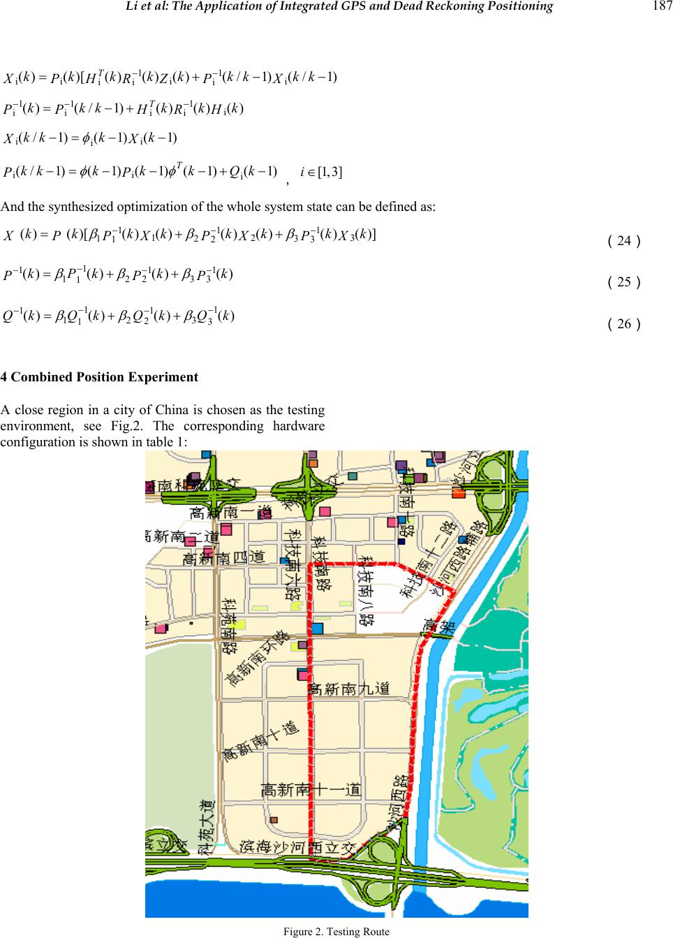

Li et al: The Application of Integrated GPS and Dead Reckoning Positioning 187
11
ii ii
ii i
()()[()()()( /1)( /1)
T
kkkkk kkkk
XPHRZP X
−−
=+−−
11 1
i
ii ii
()(/1)()()()
T
kkkkkk
PP HRH
−− −
=−+
ii
i
(/1)(1)(1)kkkk
XX
φ −= −−
ii
i
(/1)( 1)( 1)( 1)( 1)
T
kkk kkk Q
PP
φφ −= −−−+−， [1, 3]i
∈
And the synthesized optimization of the whole system state can be defined as:
11 1
123 12 3
123
()()[() ()()()()()]kk kkkkkk
X PPXPXPX
ββ β
−−−
=++
（24）
1
111
23 123
1
() ()()()kkkkP
PPP
βββ
−
−−−
=+ + （25）
1 1 11
23 12
13
()()() ()kkkQkQ
QQ
βββ
− − −−
=+ + （26）
4 Combined Position Expe r iment
A close region in a city of China is chosen as the testing
environment, see Fig.2. The corresponding hardware
configuration is shown in table 1:
Figure 2. Testing Route

188 Journal of Global Positioning Systems
Tab. 1 List of hardware collocations for test.
Item Configuration
main frequency 166MHz
chip SH4
memory 64M
CF card 128M
GPS Gamin 15
GYRO Matsushita
Vehicle Buick commercial
Tab. 2 The Parameters of Positioning Equipments
Parameters related to positioning equipment are shown in
Table 2. The positioning state of GPS receiver is checked
here. Fig. 3 shows the drift track of GPS positioning at a
given position over a long period of time; Fig. 4 is the
satellite distribution. In Fig. 3, we can see that the
positioning state of GPS is not satisfactory, and there are
noticeable drifts. The satellite visibility of the GPS
module is satisfactory. In most cases, it allows for
simultaneous visibility of 4 satellites with distinct signals.
Thereby after filtering processing, GPS Observation can
meet the requirements for dynamic vehicle navigation.
Fig 3. GPS Positioning Drift
Fig. 4 Satellite Distribution
Figs.5-8 illustrate the deviation between recorded track
and road feature points in different cases. Whether based
on standalone GPS positioning or the integrated
GPS/DR/MM positioning, accuracy of positioning in X-
axis or Y-axis direction is not significant. But the
deviations of positioning based on the two different
methods are distinct. The positioning error of points can
be greatly improved after GPS/DR/MM matching
(normally the method can make the accuracy increase by
30%). In rare cases there will be large matching errors.
This is mainly because, in the crossroads, there are
several choices, and various values can be obtained with
the map matching algorithm. According to the
optimization rules, the most possible road is chosen based
only on the signal value matching.
22. 522
22. 524
22. 526
22. 528
22. 53
22. 532
22. 534
22. 536
22. 538
22. 54
22. 542
113.94113.94
5
113.95113.95
5
GPS
ROAD
GPS/ DR/MM
Fig 5. Trajectory
The navigation test program of integrated GPS/DR/MM
positioning model is realized in this paper based on
item Parameter
GPS
Positioning precision <50m Normally
Startup time 20s
GYRO
Sensitivity [22.5,27.5]mV/( 1
.s
−
D)
Sensitivity drift [-5.0% ,5.0%]
Zero Point Drift [-10% ,10%]
Linearity [-5.0% ,5.0%]
Working temperature [-40,85] C
D

Li et al: The Application of Integrated GPS and Dead Reckoning Positioning 189
WinCE operation systems, and in the experiment the
vehicle moving tracks in various cases are recorded. It is
obvious that in comparatively straight places whether
single GPS positioning or integrated GPS/DR/MM
positioning is adopted we can always get well matched
results. In the curved road section, however, there will be
distinct deviations if we use standalone GPS positioning
model which can be greatly improved with integrated
GPS/DR/MM model.
5 Conclusion s
To solve the positioning problem in the vehicle
navigation, a universal model of integrated GPS/DR/MM
positioning is discussed in this paper. In the cities, it is
important to improve GPS positioning precision by the
model in the cases when GPS positioning signals are too
weak, such as in the downtown areas, tunnels,
underpasses, crossroads, etc. Obviously, forming the
model will take up computing resources of the system
more or less and the interaction with navigation digital
map is frequent. The setting of the parameters of this
model depends on experience to some extent, so
appropriate parameters can be determined only after
many trials. These parameters are quite different in digital
map databases with different precisions. In the future
study, we will consider the design and application of an
adaptive positioning model
X
113. 94
113. 942
113. 944
113. 946
113. 948
113. 95
113. 952
113. 954
13579111315 1719 21
GPS
ROAD
GPS/ DR/ MM
Fig 6. Deviation in X-axis
Y
22. 515
22. 52
22. 525
22. 53
22. 535
22. 54
22. 545
13579111315171921
GPS
ROAD
GPS/ DR/ MM
Fig 7. Deviation in Y-axis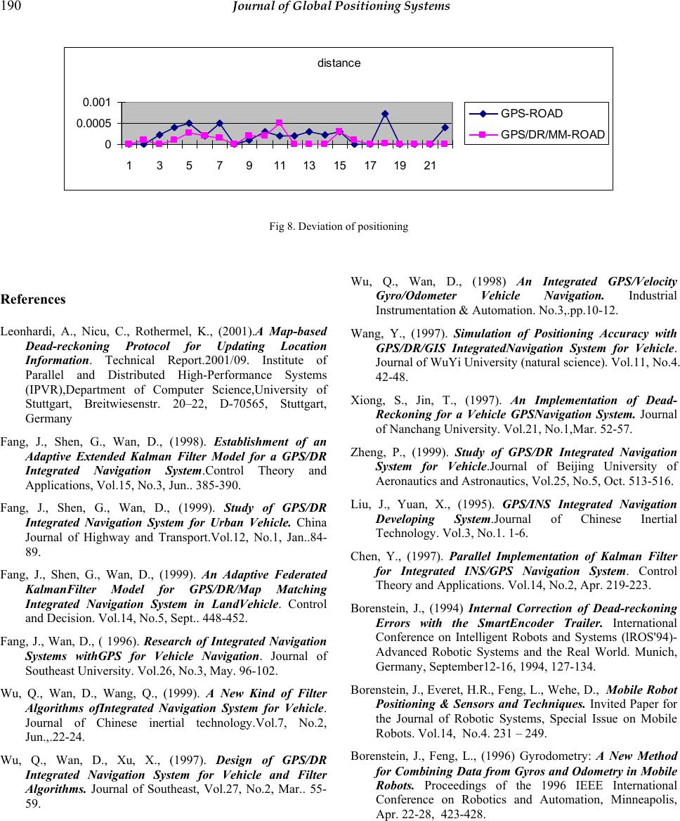

190 Journal of Global Positioning Systems
distance
0
0.0005
0.001
13 57 9111315171921
GPS-ROAD
GPS/DR/MM-ROAD
Fig 8. Deviation of positioning
References
Leonhardi, A., Nicu, C., Rothermel, K., (2001).A Map-based
Dead-reckoning Protocol for Updating Location
Information. Technical Report.2001/09. Institute of
Parallel and Distributed High-Performance Systems
(IPVR),Department of Computer Science,University of
Stuttgart, Breitwiesenstr. 20–22, D-70565, Stuttgart,
Germany
Fang, J., Shen, G., Wan, D., (1998). Establishment of an
Adaptive Extended Kalman Filter Model for a GPS/DR
Integrated Navigation System.Control Theory and
Applications, Vol.15, No.3, Jun.. 385-390.
Fang, J., Shen, G., Wan, D., (1999). Study of GPS/DR
Integrated Navigation System for Urban Vehicle. China
Journal of Highway and Transport.Vol.12, No.1, Jan..84-
89.
Fang, J., Shen, G., Wan, D., (1999). An Adaptive Federated
KalmanFilter Model for GPS/DR/Map Matching
Integrated Navigation System in LandVehicle. Control
and Decision. Vol.14, No.5, Sept.. 448-452.
Fang, J., Wan, D., ( 1996). Research of Integrated Navigation
Systems withGPS for Vehicle Navigation. Journal of
Southeast University. Vol.26, No.3, May. 96-102.
Wu, Q., Wan, D., Wang, Q., (1999). A New Kind of Filter
Algorithms ofIntegrated Navigation System for Vehicle.
Journal of Chinese inertial technology.Vol.7, No.2,
Jun.,.22-24.
Wu, Q., Wan, D., Xu, X., (1997). Design of GPS/DR
Integrated Navigation System for Vehicle and Filter
Algorithms. Journal of Southeast, Vol.27, No.2, Mar.. 55-
59.
Wu, Q., Wan, D., (1998) An Integrated GPS/Velocity
Gyro/Odometer Vehicle Navigation. Industrial
Instrumentation & Automation. No.3,.pp.10-12.
Wang, Y., (1997). Simulation of Positioning Accuracy with
GPS/DR/GIS IntegratedNavigation System for Vehicle.
Journal of WuYi University (natural science). Vol.11, No.4.
42-48.
Xiong, S., Jin, T., (1997). An Implementation of Dead-
Reckoning for a Vehicle GPSNavigation System. Journal
of Nanchang University. Vol.21, No.1,Mar. 52-57.
Zheng, P., (1999). Study of GPS/DR Integrated Navigation
System for Vehicle.Journal of Beijing University of
Aeronautics and Astronautics, Vol.25, No.5, Oct. 513-516.
Liu, J., Yuan, X., (1995). GPS/INS Integrated Navigation
Developing System.Journal of Chinese Inertial
Technology. Vol.3, No.1. 1-6.
Chen, Y., (1997). Parallel Implementation of Kalman Filter
for Integrated INS/GPS Navigation System. Control
Theory and Applications. Vol.14, No.2, Apr. 219-223.
Borenstein, J., (1994) Internal Correction of Dead-reckoning
Errors with the SmartEncoder Trailer. International
Conference on Intelligent Robots and Systems (lROS'94)-
Advanced Robotic Systems and the Real World. Munich,
Germany, September12-16, 1994, 127-134.
Borenstein, J., Everet, H.R., Feng, L., Wehe, D., Mobile Robot
Positioning & Sensors and Techniques. Invited Paper for
the Journal of Robotic Systems, Special Issue on Mobile
Robots. Vol.14, No.4. 231 – 249.
Borenstein, J., Feng, L., (1996) Gyrodometry: A New Method
for Combining Data from Gyros and Odometry in Mobile
Robots. Proceedings of the 1996 IEEE International
Conference on Robotics and Automation, Minneapolis,
Apr. 22-28, 423-428.