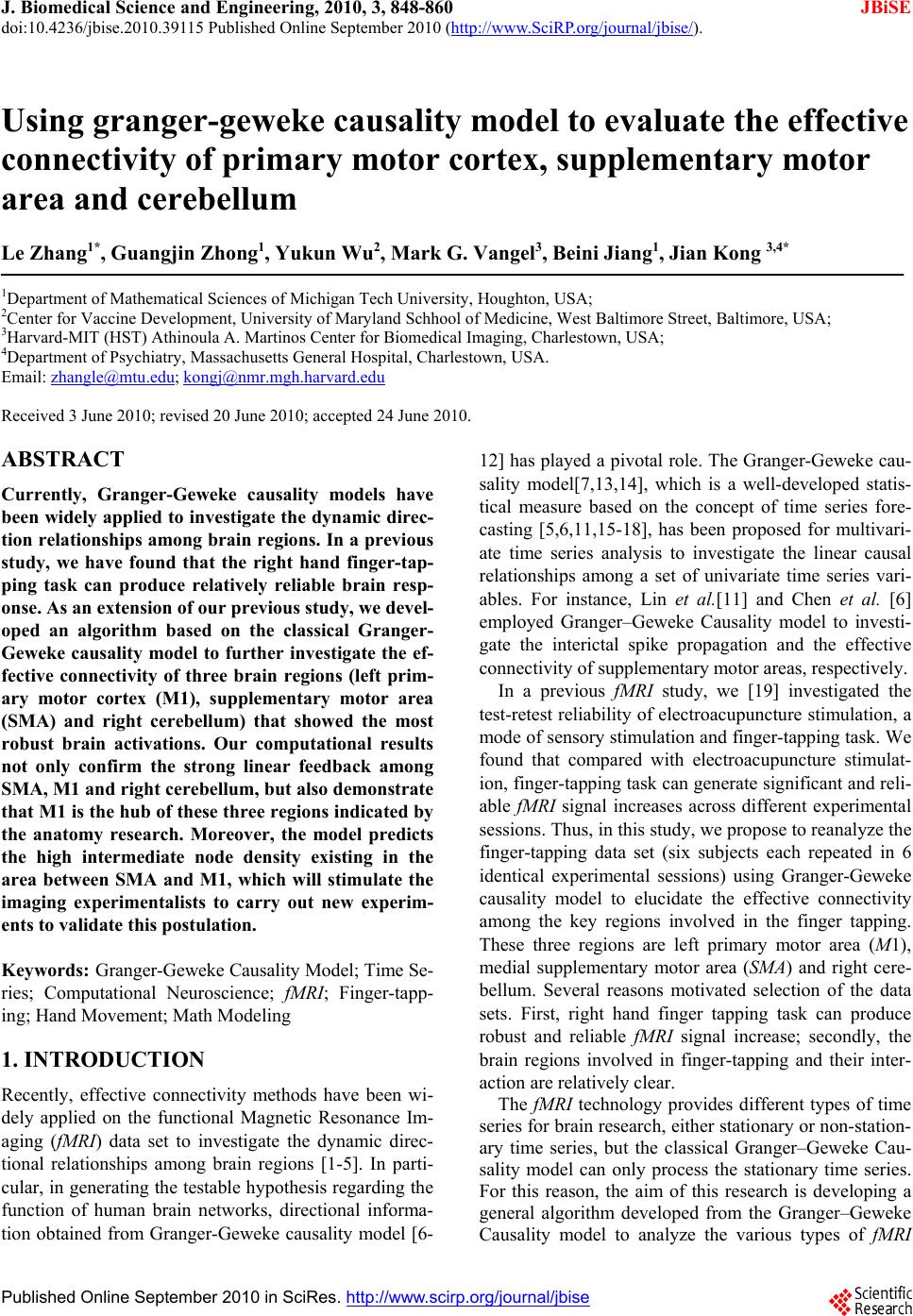
J. Biomedical Science and Engineering, 2010, 3, 848-860
doi:10.4236/jbise.2010.39115 Published Online September 2010 (http://www.SciRP.org/journal/jbise/
JBiSE
).
Published Online September 2010 in SciRes. http:// www.scirp.org/journal/jbise
Using granger-geweke causality model to evaluate the effective
connectivity of primary motor cortex, supplementary motor
area and cerebellum
Le Zhang1*, Guangjin Z hong 1, Yukun Wu2, Mark G. Vangel3, Beini Jiang1, Jian Kong 3,4*
1Department of Mathematical Sciences of Michigan Tech University, Houghton, USA;
2Center for Vaccine Development, University of Maryland Schhool of Medicine, West Baltimore Street, Baltimore, USA;
3Harvard-MIT (HST) Athinoula A. Martinos Center for Biomedical Imaging, Charlestown, USA;
4Department of Psychiatry, Massachusetts General Hospital, Charlestown, USA.
Received 3 June 2010; revised 20 June 2010; accepted 24 June 2010.
ABSTRACT
Currently, Granger-Geweke causality models have
been widely applied to investigate the dynamic direc-
tion relationships among brain regions. In a previous
study, we have found that the right hand finger-tap-
ping task can produce relatively reliable brain resp-
onse. As an extension of our previous study, we devel-
oped an algorithm based on the classical Granger-
Geweke causality model to further investigate the ef-
fective connectivity of three brain regions (left prim-
ary motor cortex (M1), supplementary motor area
(SMA) and right cerebellum) that showed the most
robust brain activations. Our computational results
not only confirm the strong linear feedback among
SMA, M1 and right cerebellum, but also demonstrate
that M1 is the hub of these three regions indicated by
the anatomy research. Moreover, the model predicts
the high intermediate node density existing in the
area between SMA and M1, which will stimulate the
imaging experimentalists to carry out new experim-
ents to validate this postulation.
Keywords: Granger-Geweke Causality Model; Time Se-
ries; Computational Neuroscience; fMRI; Finger-tapp-
ing; Hand Movement; Math Modeling
1. INTRODUCTION
Recently, effective connectivity methods have been wi-
dely applied on the functional Magnetic Resonance Im-
aging (fMRI) data set to investigate the dynamic direc-
tional relationships among brain regions [1-5]. In parti-
cular, in generating the testable hypothesis regarding the
function of human brain networks, directional informa-
tion obtained from Granger-Geweke causality model [6-
12] has played a pivotal role. The Granger-Geweke cau-
sality model[7,13,14], which is a well-developed statis-
tical measure based on the concept of time series fore-
casting [5,6,11,15-18], has been proposed for multivari-
ate time series analysis to investigate the linear causal
relationships among a set of univariate time series vari-
ables. For instance, Lin et al.[11] and Chen et al. [6]
employed Granger–Geweke Causality model to investi-
gate the interictal spike propagation and the effective
connectivity of supplementary motor areas, respectively.
In a previous fMRI study, we [19] investigated the
test-retest reliability of electroacupuncture stimulation, a
mode of sensory stimulation and finger-tapping task. We
found that compared with electroacupuncture stimulat-
ion, finger-tapping task can generate significant and reli-
able fMRI signal increases across different experimental
sessions. Thus, in this study, we propose to reanalyze the
finger-tapping data set (six subjects each repeated in 6
identical experimental sessions) using Granger-Geweke
causality model to elucidate the effective connectivity
among the key regions involved in the finger tapping.
These three regions are left primary motor area (M1),
medial supplementary motor area (SMA) and right cere-
bellum. Several reasons motivated selection of the data
sets. First, right hand finger tapping task can produce
robust and reliable fMRI signal increase; secondly, the
brain regions involved in finger-tapping and their inter-
action are relatively clear.
The fMRI technology provides different types of time
series for brain research, either stationary or non-station-
ary time series, but the classical Granger–Geweke Cau-
sality model can only process the stationary time series.
For this reason, the aim of this research is developing a
general algorithm developed from the Granger–Geweke
Causality model to analyze the various types of fMRI

L. Zhang et al. / J. Biomedical Science and Engineering 3 (2010) 848-860
849
time series, such as our previous experimental data [19].
This algorithm is briefly described as follows. First,
since fMRI will provide us a stationary or nonstationary
time series, the augmented Dickey-Fuller (ADF) unit
root test [20-22] will be implemented to test the station-
arity of raw data. If the data are nonstationary, the plot
of autocorrelation function will be applied to check the
patterns and choose an appropriate smoothing technique
to transform the raw data to stationary data. Next, the
approximation to the critical values of Schwarz’s
Bayesian information criterion (SBIC) is computed by
ARFIT algorithm [23] to determine the order of auto-
regressive equation of the Granger–Geweke Causality
model. Consequently, a time series autoregressive model
with appropriate order will be developed to fit smoothed
fMRI data. Lastly, the confidence intervals will be con-
structed for the measures of feedback. In the study, the
results of the model not only agree with our previous
experimental findings [19] that there are strong correla-
tions among SMA, M1 and cerebellum, but also match
the observations of the anatomy [24] that both SMA and
cerebellum project to M1.
2. MATERIALS AND METHODS
2.1. Experimental Material and Methods
In the present study, we reanalyzed the data from a prev-
ious study (experimental details described in the original
paper). In summary, 6 healthy right hand subjects were
included in this study. All experiments were conducted
with the written consent of each subject and approved by
the Massachusetts General Hospital’s Institutional Re-
view Board.
2.2. Experimental Procedures
Each subject participated in 6 identical fMRI scanning
sessions. Sessions 1 and 2 were separated by 20-30 min-
utes. Sessions 2 and 3 were separated by 3-6 days. After
Session 3, the interval between subsequent sessions was
7-21 days. The block design was applied. The fMRI scan
started with 30s baseline, four 30s blocks of stimulation
(ON, right finger-tapping), were separated by four rest
periods (OFF) of 30s, 60s, 30s and 30s respectively (ple-
ase see Figure 1(a) in our previous paper [19] for more
detailed experimental paradigm).
2.3. fMRI Data Acquisition and Analysis
All brain imaging was performed with a 3-axis gradient
head coil in a 3 Tesla Siemens MRI System (Erlagen,
Germany) equipped for echo planar imaging. After aut-
omated scout and shimming procedures, functional MR
images were acquired using gradient echo T2*-weighted
sequence with TR 2000 ms, TE 40 msec and a flip angle
of 90 degrees. Thirty slices (4 mm thick, 1 mm skip) ori-
ented parallel to the AC-PC plane were collected to pro-
vide whole brain coverage. A high resolution 3D MP-
RAGE sequence was also collected. Pre-processing and
statistical analysis were performed using SPM2 software
(Wellcome Department of Cognitive Neurology). Pre-
processing began with motion correction. All functional
runs were realigned to the first volume acquired in the
scan session. We set a movement threshold of 2 mm wi-
thin a scan to eliminate subjects with excessive head mo-
vement. However, none of the subjects had head move-
ments that exceeded this threshold. Thus, all data were
used for this analysis. All functional runs were normal-
ized to MNI stereotactic space and spatially smoothed
with an 8mm Gaussian kernel. A separate general linear
model (GLM) for each session was specified across each
subject with regressors for the difference from baseline
[25]. Global signal scaling was applied. Low-frequency
noise was removed with a high-pass filter applied with
default values (120 second) to the fMRI time series at
each voxel. For each individual session, a threshold of p
< 0.005 uncorrected with 10 contiguous voxels was used
for finger-tapping; then for each predefined ROI, left M1,
SMA and right cerebellum, we performed Granger cau-
sality analysis on the average time courses of voxels in 3
distinct regions, with each region defined by extracting a
sphere of radius 3mm around the peak activation voxel.
3. MATHEMATICAL MODEL
3.1. Granger-Geweke Causality Model
In this study, the Granger–Geweke Causality model is
employed as the major tool to analyze the fMRI imaging
data and to reveal the relationships among those brain
regions of interest. Consider two zero-mean vector time-
series X and Y. The time-indexed observations are de-
noted as t and t, where is the time index.
X, Y can be modeled as autoregressive (AR) processes of
order p as
x ynt ,...,1

 p
i
titit uxax
1
11 , (1)

 p
i
titit vyby
1
11 , (2)


 p
i
p
i
titiitit uycxax
11
222 , (3)


 p
i
p
i
titiitit vydxby
11
222 , (4)
where i, i1, , , , are coefficients of
AR models, and t, t, t, are the zero-mean
residuals. Their variances are , , 2, 2, re-
spectively. Let , , , be the re-
a1bi a2
u1
kn
U
1
i
b2
v1
n
V1
i
c2
u2
lU
i
d2
t
v2
1
Σ
kn
2
1
Τ
V
Σ
ln
Τ
2

L. Zhang et al. / J. Biomedical Science and Engineering 3 (2010) 848-860
850
spective residual matrix of Eq.1 through 4, the varianc-
es can be estimated by ordinary least squares (OLS)
method, such that,
/nUUΣT
111 /nVVΤT 111

2
Σ
, 22 . Then the measure of linear
feedback is computed by Eq.5 and 6.
/nUUT22
F
nV /
2
|/|ln(| 1
|/|ln(| 21 
F
|||ln(|22
VT 
XY
F
YX
F
|)
|)
|)| 
in Eq.9:
YXXYYXYXFFFF , (9)
Typically, a time series can be described as either sta-
tionary or non-stationary, depending on the constancy of
its statistical properties [26-28]. The stationary time series
should have constant mean and variance over time as
well as covariance which is a function of time difference
only. The non-stationary time series may have either
non-constant means, or non-constant variance or both,
which results in spurious regression; [29, 30]. This poses
a very serious problem for the estimation, and over- re-
jects hypothesis with T (true) or F (false) test statistics.
Since Granger-Geweke Causality model focuses on the
stationary purely nondeterministic multiple time series,
the raw fMRI imaging data is confirmed to be stationary.
If non-stationary, differencing method is employed to
transform the non-stationary data to stationary data. For
this reason, a general procedure to employ Granger-
Geweke Causality model is presented and described by
Figure 1. Next, we will illustrate each step in detail.
2, (5)
, (6)
where XY  indicates the strength of time series Y
Granger-causing X , andYX indicates the strength of
time series X Granger-causing Y. The measure of instan-
taneous linear feedback is computed by Eq.7.

T














2
2
2
C v
u
t
t


FYX
 var
/ (7)
where Г in Eq.8 is the covariance matrix




2
C
2v2
(8)
and C denotes the covariance of t, t. The measure
of linear dependence is the sum of the measures of the
three types of linear feedback, which is referred as
u
YX
F,
Figure 1. A general procedure to employ Granger-Geweke Causa-
lity model to investigate the relations among the interesting re-
gions of the brain.
JBiSE

L. Zhang et al. / J. Biomedical Science and Engineering 3 (2010) 848-860
851
3.2. Check if the Dataset are Stationary or
Non-Stationary
The augmented Dickey-Fuller (ADF) unit root test [20,
21] and the plot of autocorrelation function (ACF) [28,
31] are most two common methods to test whether the
dataset is stationary or non-stationary.
The ADF test statistics a numeric indicator such that
the more negative it is, the stronger the rejection of the
null hypothesis that there is a unit root (Data is not sta-
tionary) at some level of confidence. The ADF test mo-
del, referred as a random walk, is described by Eq.10,
t
k
j
jtjtt xxtx
  
 2
1 (10)
where k is the lag order, t
x, 1t xjt xare respective
observations at time jttt,

 ,1 , ,k,j2, in the
time series X,

is the constant drift, t

is the time-
trend term,

,

are coefficients, and t

is the noise
with mean zero and constant variance. Since the well-de-
veloped auto regression (AR) models of Granger-Ge-
weke causality model have neither time trend nor drift
processes, the current ADF test model can be simplified
as Eq.11,
t
k
j
jtjtt xxx
  
 2
1 (11)
The number of lags is determined by the sampling
frequency. If the sampling frequency is large, k should
be small [32]. Because the time frequency of the fMRI
experiments is 2 seconds long, we have to set k to 1,
smallest lag number in this case. And then the unit root
test is carried out under the null hypothesis 1


aga-
inst the alternative hypothesis of1

. Once a value for
the test statistic, Eq.12 is computed, which can be com-
pared to the relevant critical value derived in Monte
Carlo study [22]
)(/)1(
 
 SEDF (12)
If the test statistic is smaller (this test is non symmetri-
cal so we do not consider an absolute value) than the cri-
tical value at α significant level, then the null hypothesis
of γ = 1 is rejected and no unit root is present which
means the data are stationary. Once the test results (Ta-
ble 1) show that all fMRI time series are non-stationary,
the next step is to choose the appropriate smoothing
technique by ACF plot.
The ACF plot is a powerful graphical tool to measure
the correlation between observations at different dis-
tances apart, to check the randomness of data and to find
re- peating pattern in them. Given the time series X
given in Eq.1, the ACF between its observations
and is defined as
t
x
t-i
x
2
i-tt, /),cov( xitt xx




(13)
Table 1. ADF test results for time series M1, SMA and cerebellum.
Subject Session M1 SMA cerebellum SubjectSession M1 SMA cerebellum
S1 0.6283 0.6988 0.7338 S1 0.6256 0.8848 0.8332
S2 0.8834 0.7967 0.8406 S2 0.6981 0.7002 0.842
S3 0.6915 0.7164 0.6593 S3 0.7063 0.7429 0.9074
S4 0.6321 0.524 0.6405 S4 -0.113 -0.27 -0.1072
S5 0.5759 0.8567 0.8247 S5 0.8579 0.7953 0.7811
1
S6 0.7728 0.7533 0.9337
4
S6 0.7594 0.9034 0.8619
S1 0.7697 0.6838 0.7179 S1 0.7073 0.7633 0.7659
S2 0.5857 0.6571 0.6015 S2 0.8368 0.8408 0.8512
S3 0.7462 0.7352 0.7248 S3 0.6926 0.8152 0.8125
S4 0.6697 0.7857 0.7402 S4 0.7143 0.7667 0.7999
S5 0.6079 0.585 0.7134 S5 0.6698 0.7242 0.6612
2
S6 0.6473 0.6664 0.8495
5
S6 0.8022 0.8728 0.8255
S1 0.7059 0.8223 0.8381 S1 0.5849 0.8409 0.6631
S2 0.6882 0.7747 0.7634 S2 0.807 0.7644 0.84
S3 0.6972 0.8879 0.7782 S3 0.6915 0.7164 0.6593
S4 0.8751 0.782 0.6341 S4 0.7688 0.5515 0.8083
S5 0.6204 0.7089 0.6091 S5 0.6908 0.6905 0.7162
3
S6 0.7709 0.8331 0.8759
6
S6 0.7811 0.8398 0.8479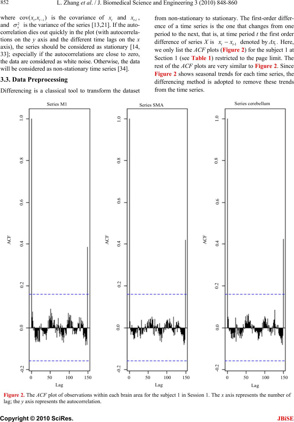

L. Zhang et al. / J. Biomedical Science and Engineering 3 (2010) 848-860
852
where is the covariance of t and t-i,
and
)(covitt ,xx 
2
x
xx

is the variance of the series [13,21]. If the auto-
correlation dies out quickly in the plot (with autocorrela-
tions on the y axis and the different time lags on the x
axis), the series should be considered as stationary [14,
33]; especially if the autocorrelations are close to zero,
the data are considered as white noise. Otherwise, the data
will be considered as non-stationary time series [34].
3.3. Data Preprocessing
Differencing is a classical tool to transform the dataset
from non-stationary to stationary. The first-order differ-
ence of a time series is the one that changes from one
period to the next, that is, at time period t the first order
difference of series X is denoted byt. Here,
we only list the ACF plots (Figure 2) for the subject 1 at
Section 1 (see Table 1) restricted to the page limit. The
rest of the ACF plots are very similar to Figure 2. Since
Figure 2 shows seasonal trends for each time series, the
differencing method is adopted to remove these trends
from the time series.
1t-t xxΔx
Series M1 Series SMASeries cerebellum
ACF
ACF
ACF
1.0
0.8
0.6
0.4
0.2
0.0
-0.2
-0.2
-0.2
Lag Lag Lag
0 50 100 150 0 50 100 150 0 50 100 150
0.0
0.0
0.2
0.2
0.4
0.4
0.6
0.6
0.8 0.8
1.0
1.0
Figure 2. The ACF plot of observations within each brain area for the subject 1 in Session 1. The x axis represents the number of
lag; the y axis represents the autocorrelation.

L. Zhang et al. / J. Biomedical Science and Engineering 3 (2010) 848-860
853
Therefore, the Eq.1 through Eq.4 can be rewritten as

 p i
titit uΔxaΔx
1
11 (14)


 p
i
titit vΔybΔy
1
11 (15)


  p
i
p
i
titiitit uΔycΔxaΔx
11
222 (16)


 p
i
p
i
titiititvΔydΔxbΔy
11
222 (17)
After the first-order difference, ADF test is employed
again of t to evaluate whether the treated dataset is
stationary or non-stationary. If it is still non-stationary,
the second-order difference (21 )
should be applied. However, if the series need different-
ing more than twice we should use other methods, such
as log transformation. In the results section of the study,
we are going to discuss the data preprocessing result in
detail.
Δx
22tttt xxxx
3.4. Model Selection
After the stationary data set is generated, the order of the
Eq.14 to 17 by computing the approximation to the cri-
teria values of Schwarz's Bayesian information criterion
(SBIC) is identified with ARFIT algorithm [23,35]. SBIC
is an information criterion used for goodness-of-fit mod-
el selection for fixed effects models with different num-
ber of parameters at some significance level, and the one
with lower SBIC fits the data better. The SBIC is descry-
bed as Eq.18.
nkLSBIC lnln2 


(18)
where n is the number of observations, k is the number
of free parameters to be estimated, and L is the maxim-
ized value of the likelihood function for the estimated
model.
3.5. Linear Feedback Calculation
After the order of AR models is determined, the linear feed-
back for each pair of brain regions by Eq.5 and 6 is
computed. Then, the conventional large-sample distribu-
tion theory is used to test the null hypothesis that a given
measure of feedback zero. As indicated by Geweke’s
research[7] if 0

XY
F, then ; if )(~
ˆ2klpFn XY



0

YX
F, then ; if )klp 0 (
2
 ~
ˆ
Fn XY



YX
F
0,~
ˆ

YX
Fn
, then
; if , then
)kl X F(
2
~
ˆ
Fn YX 


))12((
, Y
2


pkl . The k, l are the number of columns in the
residual matrix, . And p is the lag of autor-
kn
U
1ln
V
1
egressive models. With respect to this null hypothesis
test, we can have the following eight relations
(Eqs.19.1-19.8) between two series X and Y [36] de-
scribed by Figure 3.
Relations Sign equation
X and Y are independent, if . 0
, YX
F(x, y) (19.1)
Instantaneous causality only without direction, if 0,0,0
,



 YXXYYXFFF . (x − y) (19.2)
X causes Y, with instantaneous causality, if 0,0,0
,



 YXXYYXFFF (x → y) (19.3)
X causes Y, without instantaneous causality, if 0,0,0
,



 YXXYYXFFF (x => y) (19.4)
Y causes X, with instantaneous causality, if 0,0,0
,



 YXXYYX FFF (x ← y) (19.5)
Y causes X, without instantaneous causality, if 0,0,0
,



 YXXYYX FFF (x <= y) (19.6)
Feedback with instantaneous causality, if 0,0,0
,



YXXYYX FFF (x ↔ y) (19.7)
Feedback without instantaneous causality 0,0,0
,



 YXXYYX FFF (x  y) (19.8)
4. RESULTS
Stationary check for the dataset: Table 1 shows the ADF
test results for time series M1, SMA, and cerebellum. It
indicates that each time series is non-stationary at 10%
significant level. Figure 2 shows the ACF plots of each
time series for subject 1 at session 1 and the ACF plots
of the rest of persons are similar with Figure 2. For this
reason, we should employ differencing method to trans-
form the dataset from non-stationary to stationary time
series.
Data transformation from non-stationary to stationary
time series: Table 2 shows ADF test results for time ser-
ies M1, SMA, and cerebellum after the first-order differe-
ncing method is applied. Now each time series is stationary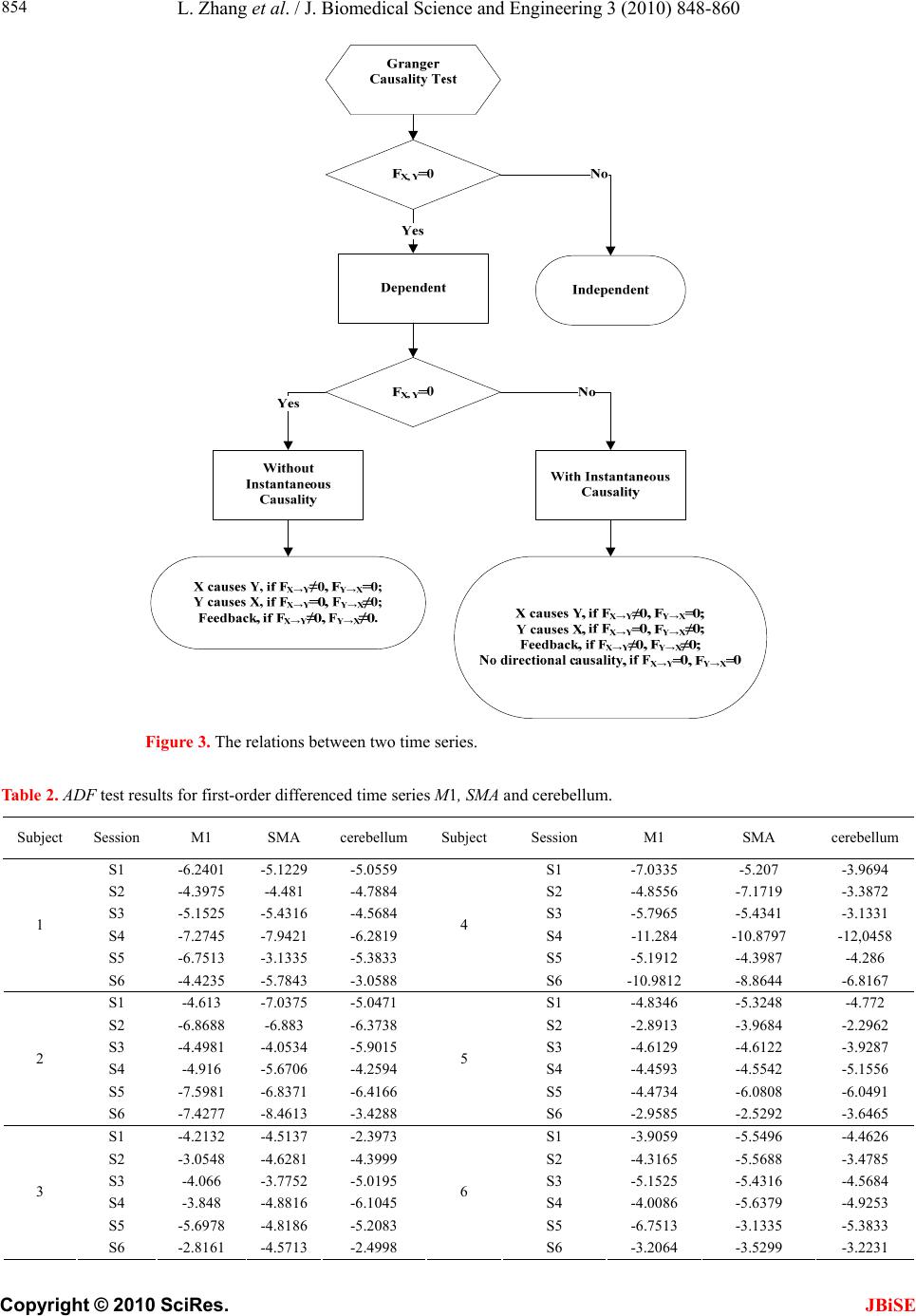

L. Zhang et al. / J. Biomedical Science and Engineering 3 (2010) 848-860
854
Figure 3. The relations between two time series.
Table 2. ADF test results for first-order differenced time series M1, SMA and cerebellum.
Subject Session M1 SMA cerebellum Subject Session M1 SMA cerebellum
S1 -6.2401 -5.1229 -5.0559 S1 -7.0335 -5.207 -3.9694
S2 -4.3975 -4.481 -4.7884 S2 -4.8556 -7.1719 -3.3872
S3 -5.1525 -5.4316 -4.5684 S3 -5.7965 -5.4341 -3.1331
S4 -7.2745 -7.9421 -6.2819 S4 -11.284 -10.8797 -12,0458
S5 -6.7513 -3.1335 -5.3833 S5 -5.1912 -4.3987 -4.286
1
S6 -4.4235 -5.7843 -3.0588
4
S6 -10.9812 -8.8644 -6.8167
S1 -4.613 -7.0375 -5.0471 S1 -4.8346 -5.3248 -4.772
S2 -6.8688 -6.883 -6.3738 S2 -2.8913 -3.9684 -2.2962
S3 -4.4981 -4.0534 -5.9015 S3 -4.6129 -4.6122 -3.9287
S4 -4.916 -5.6706 -4.2594 S4 -4.4593 -4.5542 -5.1556
S5 -7.5981 -6.8371 -6.4166 S5 -4.4734 -6.0808 -6.0491
2
S6 -7.4277 -8.4613 -3.4288
5
S6 -2.9585 -2.5292 -3.6465
S1 -4.2132 -4.5137 -2.3973 S1 -3.9059 -5.5496 -4.4626
S2 -3.0548 -4.6281 -4.3999 S2 -4.3165 -5.5688 -3.4785
S3 -4.066 -3.7752 -5.0195 S3 -5.1525 -5.4316 -4.5684
S4 -3.848 -4.8816 -6.1045 S4 -4.0086 -5.6379 -4.9253
S5 -5.6978 -4.8186 -5.2083 S5 -6.7513 -3.1335 -5.3833
3
S6 -2.8161 -4.5713 -2.4998
6
S6 -3.2064 -3.5299 -3.2231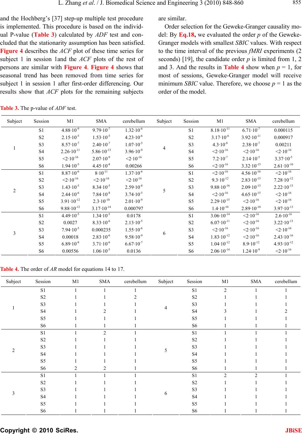

L. Zhang et al. / J. Biomedical Science and Engineering 3 (2010) 848-860
855
and the Hochberg’s [37] step-up multiple test procedure
is implemented. This procedure is based on the individ-
ual P-value (Table 3) calculated by ADF test and con-
cluded that the stationarity assumption has been satisfied.
Figure 4 describes the ACF plot of these time series for
subject 1 in session 1and the ACF plots of the rest of
persons are similar with Figure 4. Figure 4 shows that
seasonal trend has been removed from time series for
subject 1 in session 1 after first-order differencing. Our
results show that ACF plots for the remaining subjects
are similar.
Order selection for the Geweke-Granger causality mo-
del: By Eq.18, we evaluated the order p of the Geweke-
Granger models with smallest SBIC values. With respect
to the time interval of the previous fMRI experiments (2
seconds) [19], the candidate order p is limited from 1, 2
and 3. And the results in Table 4 show when p = 1, for
most of sessions, Geweke-Granger model will receive
minimum SBIC value. Therefore, we choose p = 1 as the
order of the model.
Table 3. The p-value of ADF test.
Subject Session M1 SMA cerebellum Subject Session M1 SMA cerebellum
S1 4.88·10-9 9.79·10-7 1.32·10-6 S1 8.18·10-11 6.71·10-7 0.000115
S2 2.15·10-5 1.53·10-5 4.23·10-6 S2 3.17·10-6 3.92·10-11 0.000917
S3 8.57·10-7 2.40·10-7 1.07·10-5 S3 4.3·10-8 2.38·10-7 0.00211
S4 2.26·10-11 5.86·10-13 3.96·10-9 S4 <2·10-16 <2·10-16 <2·10-1 6
S5 <2·10-16 2.07·10-9 <2·10-16 S5 7.2·10-7 2.14·10-5 3.37·10-5
1
S6 1.94·10-5 4.45·10-8 0.00266
4
S6 <2·10-16 3.32·10-15 2.61·10-10
S1 8.87·10-6 8·10-11 1.37·10-6 S1 <2·10-16 4.56·10-16 <2·10-16
S2 <2·10-16 <2·10-16 <2·10-16 S2 9.3·10-12 2.83·10-15 7.28·10-12
S3 1.43·10-5 8.34·10-5 2.59·10-8 S3 9.88·10-16 2.09·10-13 2.22·10-15
S4 2.44·10-6 7.84·10-8 3.74·10-5 S4 <2·10-16 4.65·10-15 <2·10-1 6
S5 3.91·10-12 2.3·10-10 2.01·10-9 S5 2.29·10-15 <2·10-16 <2·10-1 6
2
S6 9.88·10-12 3.17·10-14 0.000797
5
S6 1.4·10-10 2.89·10-10 3.97·10-13
S1 4.49·10-5 1.34·10-5 0.0178 S1 3.06·10-14 <2·10-16 2.6·10-16
S2 0.0027 8.33·10-6 2.13·10-5 S2 6.07·10-11 <2·10-16 3.22·10-13
S3 7.94·10-5 0.000235 1.55·10-6 S3 <2·10-16 <2·10-16 <2·10-1 6
S4 0.00018 2.83·10-6 9.58·10-9 S4 1.83·10-12 <2·10-1 6 2.43·10-16
S5 6.89·10-8 3.71·10-6 6.67·10-7 S5 1.04·10-12 8.9·10-12 4.93·10-12
3
S6 0.00556 1.06·10-5 0.0136
6
S6 2.06·10-14 1.24·10-9 <2·10-16
Table 4. The order of AR model for equations 14 to 17.
Subject Session M1 SMA cerebellum Subject Session M1 SMA cerebellum
S1 1 1 1 S1 2 1 1
S2 1 1 2 S2 1 1 1
S3 1 1 1 S3 1 1 1
S4 1 2 1 S4 3 1 2
S5 1 1 1 S5 1 1 1
1
S6 1 1 1
4
S6 1 1 1
S1 1 2 1 S1 1 1 1
S2 1 1 1 S2 1 1 1
S3 1 1 1 S3 1 1 1
S4 1 1 1 S4 1 1 1
S5 1 1 1 S5 1 1 1
2
S6 2 2 1
5
S6 1 1 1
S1 1 1 1 S1 2 2 1
S2 1 1 1 S2 1 1 1
S3 1 1 1 S3 1 1 1
S4 1 1 1 S4 1 1 1
S5 1 1 1 S5 1 1 1
3
S6 1 1 1
6
S6 1 1 1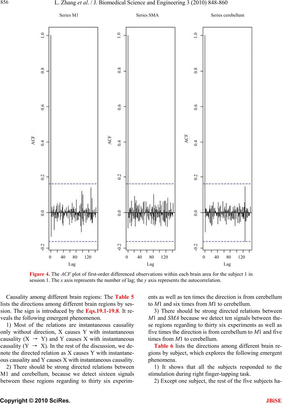

L. Zhang et al. / J. Biomedical Science and Engineering 3 (2010) 848-860
856
Series M1 Series SMASeries cerebellum
ACF
1.0 0.8 0.6 0.4 0.2 0.0 -0.2
Lag
0 40 80 120
1.0 1.0
0.8 0.6 0.4 0.2 0.0 -0.2 0.8 0.6 0.4 0.2 0.0 -0.2
ACF
ACF
0 40 80 1200 40 80 120
Lag Lag
Figure 4. The ACF plot of first-order differenced observations within each brain area for the subject 1 in
session 1. The x axis represents the number of lag; the y axis represents the autocorrelation.
Causality among different brain regions: The Table 5
lists the directions among different brain regions by ses-
sion. The sign is introduced by the Eqs.19.1-19.8. It re-
veals the following emergent phenomenon.
1) Most of the relations are instantaneous causality
only without direction, X causes Y with instantaneous
causality (X → Y) and Y causes X with instantaneous
causality (Y → X). In the rest of the discussion, we de-
note the directed relation as X causes Y with instantane-
ous causality and Y causes X with instantaneous causality.
2) There should be strong directed relations between
M1 and cerebellum, because we detect sixteen signals
between these regions regarding to thirty six experim-
ents as well as ten times the direction is from cerebellum
to M1 and six times from M1 to cerebellum.
3) There should be strong directed relations between
M1 and SMA because we detect ten signals between the-
se regions regarding to thirty six experiments as well as
five times the direction is from cerebellum to M1 and five
times from M1 to cerebellum.
Table 6 lists the directions among different brain re-
gions by subject, which explores the following emergent
phenomena.
1) It shows that all the subjects responded to the
stimulation during right finger-tapping task.
2) Except one subject, the rest of the five subjects ha-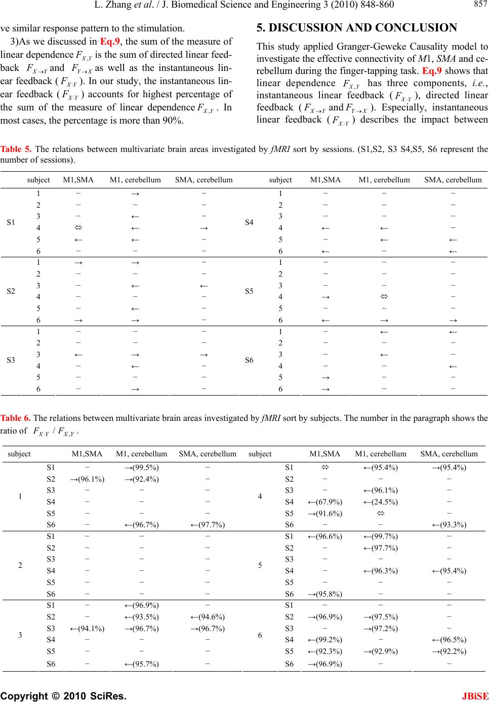

L. Zhang et al. / J. Biomedical Science and Engineering 3 (2010) 848-860
857
ve similar response pattern to the stimulation.
3)As we discussed in Eq.9, the sum of the measure of
linear dependenceis the sum of directed linear feed-
back YX and Xas well as the instantaneous lin-
ear feedback (). In our study, the instantaneous lin-
ear feedback () accounts for highest percentage of
the sum of the measure of linear dependence. In
most cases, the percentage is more than 90%.
YX
F,
Y
F
Y
Y
F
X
X
F
F
YX
F,
5. DISCUSSION AND CONCLUSION
This study applied Granger-Geweke Causality model to
investigate the effective connectivity of M1, SMA and ce-
rebellum during the finger-tapping task. Eq.9 shows that
linear dependence YX has three components, i.e.,
instantaneous linear feedback (YX ), directed linear
feedback (YX andXY ). Especially, instantaneous
linear feedback () describes the impact between
F,
F
YX 
F
F
F
Ta bl e 5. The relations between multivariate brain areas investigated by fMRI sort by sessions. (S1,S2, S3 S4,S5, S6 represent the
number of sessions).
subject M1,SMA M1, cerebellum SMA, cerebellum subject M1,SMA M1, cerebellum SMA, cerebellum
1 − → − 1 − − −
2 − − − 2 − − −
3 − ← − 3 − − −
4  ← → 4 ← ← −
5 ← ← − 5 − ← ←
S1
6 − − −
S4
6 ← − ←
1 → → − 1 − − −
2 − − − 2 − − −
3 − ← ← 3 − − −
4 − − − 4 →  −
5 − ← − 5 − − −
S2
6 → → −
S5
6 ← → →
1 − − − 1 − ← ←
2 − − − 2 − − −
3 ← → → 3 − ← −
4 − ← − 4 − − ←
5 − − − 5 → − −
S3
6 − → −
S6
6 → − −
Table 6. The relations between multivariate brain areas investigated by fMRI sort by subjects. The number in the paragraph shows the
ratio of .
YXYX FF,
/

subject M1,SMA M1, cerebellum SMA, cerebellumsubject M1,SMA M1, cerebellum SMA, cerebellum
S1 − →(99.5%) − S1 ←(95.4%) →(95.4%)
S2 →(96.1%) →(92.4%) − S2− − −
S3 − − − S3− ←(96.1%) −
S4 − − − S4←(67.9%) ←(24.5%) −
S5 − − − S5→(91.6%) −
1
S6 − ←(96.7%) ←(97.7%)
4
S6 − − ←(93.3%)
S1 − − − S1←(96.6%) ←(99.7%) −
S2 − − − S2− ←(97.7%) −
S3 − − − S3− − −
S4 − − − S4− ←(96.3%) ←(95.4%)
S5 − − − S5− − −
2
S6 − − −
5
S6 →(95.8%)− −
S1 − ←(96.9%) − S1− − −
S2 − ←(93.5%) ←(94.6%) S2→(96.9%) →(97.5%) −
S3 ←(94.1%) →(96.7%) →(96.7%) S3− →(97.2%) −
S4 − − − S4←(99.2%)− ←(96.5%)
S5 − − − S5←(92.3%) →(92.9%) →(92.2%)
3
S6 − ←(95.7%) −
6
S6 →(96.9%)− −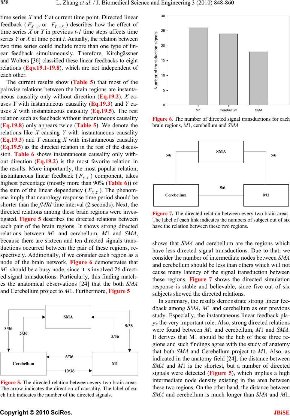

L. Zhang et al. / J. Biomedical Science and Engineering 3 (2010) 848-860
858
time series X and Y at current time point. Directed linear
feedback (YX or XY ) describes how the effect of
time series X or Y in previous t-1 time steps affects time
series Y or X at time point t. Actually, the relation between
two time series could include more than one type of lin-
ear feedback simultaneously. Therefore, Kirchgässner
and Wolters [36] classified these linear feedbacks to eight
relations (Eqs.19.1-19.8), which are not independent of
each other.
FF
The current results show (Table 5) that most of the
pairwise relations between the brain regions are instanta-
neous causality only without direction (Eq.19.2). X ca-
uses Y with instantaneous causality (Eq.19.3) and Y ca-
uses X with instantaneous causality (Eq.19.5). The rest
relation such as feedback without instantaneous causality
(Eq.19.8) only appears twice (Table 5). We denote the
relations like X causing Y with instantaneous causality
(Eq.19.3) and Y causing X with instantaneous causality
(Eq.19.5) as the directed relation in the rest of the discus-
sion. Table 6 shows instantaneous causality only with-
out direction (Eq.19.2) is the most favorite relation in
the results. More importantly, the most popular relation,
instantaneous linear feedback (YX ) component, takes
highest percentage (mostly more than 90% (Table 6)) of
the sum of the linear dependency (YX ,). The phenom-
ena imply that neurology response time period should be
shorter than the fMRI time interval (2 seconds). Next, the
directed relations among these brain regions were inves-
tigated. Figure 5 describes the directed relations between
each pair of the brain regions. It shows strong directed
relations between M1 and cerebellum, M1 and SMA,
because there are sixteen and ten directed signals trans-
ductions occurred between the pair of these regions, re-
spectively. Additionally, if we consider each region as a
node of the brain network, Figure 6 demonstrates that
M1 should be a busy node, since it is involved 26 direct-
ed signal transductions. Particularly, this finding match-
es the anatomical observations [24] that the both SMA
and Cerebellum project to M1. Furthermore, Figure 5
F
F
Figure 5. The directed relation between every two brain areas.
The arrow indicates the direction of causality. The label of ea-
ch link indicates the number of the directed signals.
M1Cerebellum SMA
Number of transduction signals
0
5
10
15
20
25
30
Figure 6. The number of directed signal transductions for each
brain regions, M1, cerebellum and SMA.
Figure 7. The directed relation between every two brain areas.
The label of each link indicates the numbers of subject out of six
have the relation between these two regions.
shows that SMA and cerebellum are the regions which
have less directed signal transductions. Due to that, we
consider the number of intermediate nodes between SMA
and cerebellum should be less than others which will not
cause many latency of the signal transduction between
these regions. Figure 7 shows the directed simulation
response is stable and believable, since five out of six
subjects showed the directed relations.
In summary, the results demonstrate strong linear fee-
dback among SMA, M1 and cerebellum as our previous
study. Especially, the instantaneous linear feedback pla-
ys the very important role. Also, strong directed relations
were found between M1 and cerebellum, M1 and SMA.
It derives that M1 should be the hub of these three re-
gions and such findings agree with the study of anatomy
that both SMA and Cerebellum project to M1. Also, as
indicated in the anatomy field [24], the distance between
SMA and M1 is the shortest, but a number of directed
signals were detected (Figure 5), which implies a high
intermediate node density existing in the area between
these two regions. On the other hand, the distance between
SMA and cerebellum is much longer than SMA and M1,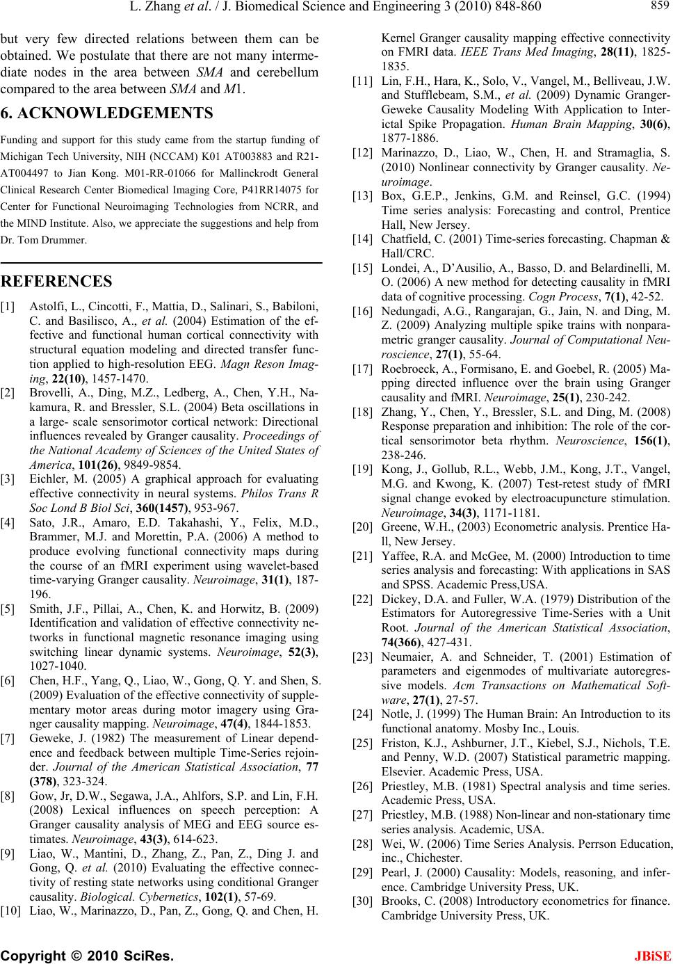

L. Zhang et al. / J. Biomedical Science and Engineering 3 (2010) 848-860
859
but very few directed relations between them can be
obtained. We postulate that there are not many interme-
diate nodes in the area between SMA and cerebellum
compared to the area between SMA and M1.
6. ACKNOWLEDGEMENTS
Funding and support for this study came from the startup funding of
Michigan Tech University, NIH (NCCAM) K01 AT003883 and R21-
AT004497 to Jian Kong. M01-RR-01066 for Mallinckrodt General
Clinical Research Center Biomedical Imaging Core, P41RR14075 for
Center for Functional Neuroimaging Technologies from NCRR, and
the MIND Institute. Also, we appreciate the suggestions and help from
Dr. Tom Drummer.
REFERENCES
[1] Astolfi, L., Cincotti, F., Mattia, D., Salinari, S., Babiloni,
C. and Basilisco, A., et al. (2004) Estimation of the ef-
fective and functional human cortical connectivity with
structural equation modeling and directed transfer func-
tion applied to high-resolution EEG. Magn Reson Imag-
ing, 22(10), 1457-1470.
[2] Brovelli, A., Ding, M.Z., Ledberg, A., Chen, Y.H., Na-
kamura, R. and Bressler, S.L. (2004) Beta oscillations in
a large- scale sensorimotor cortical network: Directional
influences revealed by Granger causality. Proceedings of
the National Academy of Sciences of the United States of
America, 101(26), 9849-9854.
[3] Eichler, M. (2005) A graphical approach for evaluating
effective connectivity in neural systems. Philos Trans R
Soc Lond B Biol Sci, 360(1457), 953-967.
[4] Sato, J.R., Amaro, E.D. Takahashi, Y., Felix, M.D.,
Brammer, M.J. and Morettin, P.A. (2006) A method to
produce evolving functional connectivity maps during
the course of an fMRI experiment using wavelet-based
time-varying Granger causality. Neuroimage, 31(1), 187-
196.
[5] Smith, J.F., Pillai, A., Chen, K. and Horwitz, B. (2009)
Identification and validation of effective connectivity ne-
tworks in functional magnetic resonance imaging using
switching linear dynamic systems. Neuroimage, 52(3),
1027-1040.
[6] Chen, H.F., Yang, Q., Liao, W., Gong, Q. Y. and Shen, S.
(2009) Evaluation of the effective connectivity of supple-
mentary motor areas during motor imagery using Gra-
nger causality mapping. Neuroimage, 47(4), 1844-1853.
[7] Geweke, J. (1982) The measurement of Linear depend-
ence and feedback between multiple Time-Series rejoin-
der. Journal of the American Statistical Association, 77
(378), 323-324.
[8] Gow, Jr, D.W., Segawa, J.A., Ahlfors, S.P. and Lin, F.H.
(2008) Lexical influences on speech perception: A
Granger causality analysis of MEG and EEG source es-
timates. Neuroimage, 43(3), 614-623.
[9] Liao, W., Mantini, D., Zhang, Z., Pan, Z., Ding J. and
Gong, Q. et al. (2010) Evaluating the effective connec-
tivity of resting state networks using conditional Granger
causality. Biological. Cybernetics, 102(1), 57-69.
[10] Liao, W., Marinazzo, D., Pan, Z., Gong, Q. and Chen, H.
Kernel Granger causality mapping effective connectivity
on FMRI data. IEEE Trans Med Imaging, 28(11), 1825-
1835.
[11] Lin, F.H., Hara, K., Solo, V., Vangel, M., Belliveau, J.W.
and Stufflebeam, S.M., et al. (2009) Dynamic Granger-
Geweke Causality Modeling With Application to Inter-
ictal Spike Propagation. Human Brain Mapping, 30(6),
1877-1886.
[12] Marinazzo, D., Liao, W., Chen, H. and Stramaglia, S.
(2010) Nonlinear connectivity by Granger causality. Ne-
uroimage.
[13] Box, G.E.P., Jenkins, G.M. and Reinsel, G.C. (1994)
Time series analysis: Forecasting and control, Prentice
Hall, New Jersey.
[14] Chatfield, C. (2001) Time-series forecasting. Chapman &
Hall/CRC.
[15] Londei, A., D’Ausilio, A., Basso, D. and Belardinelli, M.
O. (2006) A new method for detecting causality in fMRI
data of cognitive processing. Cogn Process, 7(1), 42-52.
[16] Nedungadi, A.G., Rangarajan, G., Jain, N. and Ding, M.
Z. (2009) Analyzing multiple spike trains with nonpara-
metric granger causality. Journal of Computational Neu-
roscience, 27(1), 55-64.
[17] Roebroeck, A., Formisano, E. and Goebel, R. (2005) Ma-
pping directed influence over the brain using Granger
causality and fMRI. Neuroimage, 25(1), 230-242.
[18] Zhang, Y., Chen, Y., Bressler, S.L. and Ding, M. (2008)
Response preparation and inhibition: The role of the cor-
tical sensorimotor beta rhythm. Neuroscience, 156(1),
238-246.
[19] Kong, J., Gollub, R.L., Webb, J.M., Kong, J.T., Vangel,
M.G. and Kwong, K. (2007) Test-retest study of fMRI
signal change evoked by electroacupuncture stimulation.
Neuroimage, 34(3), 1171-1181.
[20] Greene, W.H., (2003) Econometric analysis. Prentice Ha-
ll, New Jersey.
[21] Yaffee, R.A. and McGee, M. (2000) Introduction to time
series analysis and forecasting: With applications in SAS
and SPSS. Academic Press,USA.
[22] Dickey, D.A. and Fuller, W.A. (1979) Distribution of the
Estimators for Autoregressive Time-Series with a Unit
Root. Journal of the American Statistical Association,
74(366), 427-431.
[23] Neumaier, A. and Schneider, T. (2001) Estimation of
parameters and eigenmodes of multivariate autoregres-
sive models. Acm Transactions on Mathematical Soft-
ware, 27(1), 27-57.
[24] Notle, J. (1999) The Human Brain: An Introduction to its
functional anatomy. Mosby Inc., Louis.
[25] Friston, K.J., Ashburner, J.T., Kiebel, S.J., Nichols, T.E.
and Penny, W.D. (2007) Statistical parametric mapping.
Elsevier. Academic Press, USA.
[26] Priestley, M.B. (1981) Spectral analysis and time series.
Academic Press, USA.
[27] Priestley, M.B. (1988) Non-linear and non-stationary time
series analysis. Academic, USA.
[28] Wei, W. (2006) Time Series Analysis. Perrson Education,
inc., Chichester.
[29] Pearl, J. (2000) Causality: Models, reasoning, and infer-
ence. Cambridge University Press, UK.
[30] Brooks, C. (2008) Introductory econometrics for finance.
Cambridge University Press, UK.

L. Zhang et al. / J. Biomedical Science and Engineering 3 (2010) 848-860
860
JBiSE
[31] Baum, C.F. (2006) An introduction to modern economet-
rics using Stata. Stata Press, Texas.
[32] Warner, R.M. (1998) Spectral analysis of time-series
data. Guilford Press, New York.
[33] Mills, T.C. (1990) Time series techniques for economists,
Cambridge University Press, UK.
[34] Clements, P. and Hendry, D.F. (1999) Forecasting non-
stationary economic time series. MIT Press, Cambridge.
[35] Storch, H.V. and Zwiers, F.W. (1999) Statistical analysis
in climate research. Cambridge University Press, UK.
[36] Kirchgässner, G. and Wolters, J. (2007) Introduction to
modern time series analysis. Springer, New York.
[37] Hochberg, Y. (1988) A Sharper Bonferroni Procedure for
Multiple Tests of Significance. Biometrika, 75(4), 800-
802.