Paper Menu >>
Journal Menu >>
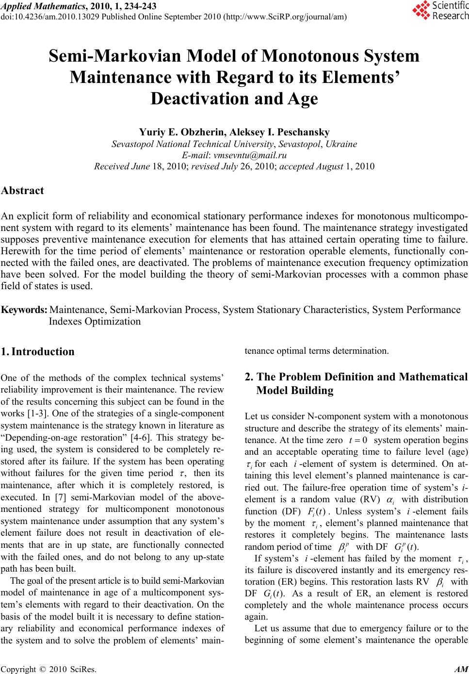 Applied Mathematics, 2010, 1, 234-243 doi:10.4236/am.2010.13029 Published Online September 2010 (http://www.SciRP.org/journal/am) Copyright © 2010 SciRes. AM Semi-Markovian Model of Monotonous System Maintenance with Regard to its Elements’ Deactivation and Age Yuriy E. Obzherin, Aleksey I. Peschansky Sevastopol National Technical University, Sevastopol, Ukraine E-mail: vmsevntu@mail.ru Received June 18, 2010; revised July 26, 2010; accepted August 1, 2010 Abstract An explicit form of reliability and economical stationary performance indexes for monotonous multicompo- nent system with regard to its elements’ maintenance has been found. The maintenance strategy investigated supposes preventive maintenance execution for elements that has attained certain operating time to failure. Herewith for the time period of elements’ maintenance or restoration operable elements, functionally con- nected with the failed ones, are deactivated. The problems of maintenance execution frequency optimization have been solved. For the model building the theory of semi-Markovian processes with a common phase field of states is used. Keywords: Maintenance, Semi-Markovian Process, System Stationary Characteristics, System Performance Indexes Optimization 1. Introduction One of the methods of the complex technical systems’ reliability improvement is their maintenance. The review of the results concerning this subject can be found in the works [1-3]. One of the strategies of a single-component system maintenance is the strategy known in literature as “Depending-on-age restoration” [4-6]. This strategy be- ing used, the system is considered to be completely re- stored after its failure. If the system has been operating without failures for the given time period , then its maintenance, after which it is completely restored, is executed. In [7] semi-Markovian model of the above- mentioned strategy for multicomponent monotonous system maintenance under assumption that any system’s element failure does not result in deactivation of ele- ments that are in up state, are functionally connected with the failed ones, and do not belong to any up-state path has been built. The goal of the present article is to build semi-Markovian model of maintenance in age of a multicomponent sys- tem’s elements with regard to their deactivation. On the basis of the model built it is necessary to define station- ary reliability and economical performance indexes of the system and to solve the problem of elements’ main- tenance optimal terms determination. 2. The Problem Definition and Mathematical Model Building Let us consider N-component system with a monotonous structure and describe the strategy of its elements’ main- tenance. At the time zero 0t system operation begins and an acceptable operating time to failure level (age) i for each i-element of system is determined. On at- taining this level element’s planned maintenance is car- ried out. The failure-free operation time of system’s i- element is a random value (RV) i with distribution function (DF) () i F t. Unless system’s i-element fails by the moment i , element’s planned maintenance that restores it completely begins. The maintenance lasts random period of time p i with DF (). p i Gt If system’s i-element has failed by the moment i , its failure is discovered instantly and its emergency res- toration (ER) begins. This restoration lasts RV i with DF (). i Gt As a result of ER, an element is restored completely and the whole maintenance process occurs again. Let us assume that due to emergency failure or to the beginning of some element’s maintenance the operable  Y. E. OBZHERIN ET AL. Copyright © 2010 SciRes. AM 235 elements that do not belong to any other up-state path are deactivated. Besides, the elements in state of ER or maintenance, the restoration of which would not result in any up-state path formation, are deactivated. The elements deactivated have the same operable level at the moment of their activation. The latter happens at the end of element’s ER or maintenance under the condi- tion of simultaneous up-state path formation. Time diagram of system operation is shown in Figure 1. Let us begin semi-Markovian (SM) model building of the system. To begin with the phase field of states should be defined. Each element of system can be in three physical states: 1 – in up state or deactivated in up state; 0 – in state of restoration or deactivated in state of restoration; 2 – in state of maintenance or deactivated in state of maintenance. System’s physical states will be indicated with a set of vectors 1 (,...,),0,1, 2;1,. Nk Ddd ddkN The component k d of vector d denotes the physical state of system’s k-element. The physical states to exhibit SM property, they should be extended. With this purpose we will indicate the number of element that was last to change its state. Let us add continuous components, denoting time peri- ods of elements’ dwelling in their states. In the code of extended state these time periods will be indicated by vector () 111 ( ,...,,0,,...,) i ii N x xx xx . Besides, in accordance with the chosen maintenance strategy we will introduce vector 1 ( ,...,), N uu u the components of which indicate elements’ operating time since the last restoration of their up state, to the code of system’s states. Thus, the system’s phase field of SM states with re- gard to its elements’ maintenance execution is the foll- owing: () ,1, i EidxuiN The significance of the code of states: i is the number of element that was last to change its physical state; 0,1,2 k d is the code of system’s k-element physi- cal state; k x is time period between i-element’s last state change and the nearest moment of k-element’s change (0) i x regardless of deactivation time; and ifk d 1 then k x is the time period till the nearest emer- gency failure of k-element; k u is operating time to failure of k-element since the end of its last ER or maintenance. If 2 k d it is considered that kk u . At the moment of i-element’s transition to up state after its maintenance or ER its op- erating time is equal zero: 0 i u. Let us indicate d I a set of numbers of elements de- activated in the state () ,1,. i id xuiN System dwelling time periods are defined by ratios: () 1 () i i d dd d ikkk ki id xuk kI kI x u where is a sign of minimum; 1 d is a set of num- bers of vector d components that are equal to 1, () ,1, ,0, ,2. i ii d iii p ii d d d Let us describe the probabilities (probability densities) of embedded Markovian chain (EMC) ,0 nn tran- sition. It is necessary to note that i-element can change its physical state 1 into the state 0 (ER) and into the 1 . . i . . N t t 0 0 0 1 N 1 1 1 i i N N N i 1 p N p 1 Figure 1. Time diagram of the system operation with elements’ deactivation after the first element failure and with regard to their maintenance in age.  Y. E. OBZHERIN ET AL. Copyright © 2010 SciRes. AM 236 state 2 (maintenance) but the states 0 and 2 can be changed only into the state 1. Let us indicate 1 ,d d dd iIkk k ki k kI kI zx u (1) and let 0 d , 2 d be sets of numbers of vector d com- ponents that are equal to 0 and 2 respectively. The state () ,1, i id xuiN admits the following transitions: 1) to the set of states () ,2 i i idxud with the pro- bability density of transition () () () , () i i id d id xu iiI id xu pzy , where,d iI y z,() () i d i , is the density of probability distribution of RV () i d i , kk dd , ki; , () d kk iI x xz y , ki, d kI; kk x x , d kI; 1 , 0 2 1 , 02 ,,, ,,,, ,, ,, 0, ; d d kiId d kk dd kd iiI d i dd uz ykkI uukkIki k uz yi u i 2) to the set of states () ,1,2 i ii id xudd with transition probability () () (), i i id xuii id xu PF where kk dd , ki ; kki xx , ki , d kI; kk x x , d kI ; 1 0 2 ,,, ,,, ,; kidd kk dd kd ukkI uukkI k 3) to the set of states () ,, j d jdxujijI with the probability density of transition () () () , (), j i id d jd xu iiI id xu pzy where 0y,kk dd ,kj , i x y , ,d kkiI x xz , ,kij , 1 , 1 02 1 , 0 2 ,,0, ,,2, 0, , ,,, ,,,. ,, d d jiIdj jj dj dd kiId d kk dd kd uz jd ujd j uz kkI uukkIkj k Let us assume that the conditions of stationary distri- bution () [8,9] existence and uniqueness for EMC ,0 nn are fulfilled. The following theorem takes place. Theorem. The stationary distribution of EMC ,0 nn is defined by the following expressions: 012 012 1 () 1 ,,0, ,, dd d dd d p k kk kkkkkkkkd i kkk i p k kk kkkkk kkkd kkk ki fuGxfuxFG xix id xufuGxfuxFG xi (2) 10 2 1 () ()() 11 1 kk k d d d d d d NN N dd d i kkii kki kk kk k dD iii ki kiki iI iI iI TFTFT (1) (0)(0) 0 ,, . k p kk kkk kkkkk kkk TFtdtTFMTFM Theorem proving. The stationary distribution of prob- abilities ()B obeys the system of integral equations [8] ,. E BdzPzB For example, the equation of this system for the state () ,0,1,;; i id id xudiNiI is as follows: , 02 ()( ) , () 0 (, mI j dd d im mm mI uj d jj j jI id xufxumdxu txjdx udt (3) 0,0,1, ;; ii d x diNiI  Y. E. OBZHERIN ET AL. Copyright © 2010 SciRes. AM 237 1 , 1,, , d d ikkmI k k kI dddkiu u By the direct substitution one can check that Formula (2) define the solution of this equation. For the state ()i id xuwe deal with 0 i d , 1 i d, 11 dd i , 00 dd i , 22 dd . Substituting (2) to the sec- ond member of Equation (3) we get the following results: 012 ,, , ddd p k kk mmImkk kmIkkkkkmI kkk km fuxfuGx ufuxFGx u , 0012 0 , mI dddd dd d up k kk jjjjkkkkk kkk jkkk jI kIk jkI g xtfufuGxtfuxFGxtdt , 201 2 0 , mI ddd d dd d up pjk k k jjkkkkk kjkk jkk k jI kIkIk j g xtfuGxtfuxFF Gxtdt 02 dd dd p k kk kk kkk kk kI kI fuGxFG x 012 ,, ddd p k kk kk kmIkkkkkmI kkk fuGxufuxFG xu 10 2 dd d dd p k kk kk kkkkkk kk k kI kI fuxfuGxFG x , 02 0 mI dd dd up k kk kk kkk kk kI kI f uG xtFG xt dt t 10 2 dd d p k kk kk kkkkkk kk k fuxfuGxFG x 10 2 () 1. dd d pi k kk iikk kkkkkk kk k ki f ufuxfuGxFGx idxu In the same way it can be checked that Formula (2) define the stationary distributions for the rest of system’s states. The constant is determined due to normaliza- tion condition. 3. Definition of System Stationary Characteristics Let us define the following system stationary perform- ance indexes: mean stationary operating time to failure 1 ( ,...,) N T ; mean stationary restoration time 1 ( ,...,) N T ; stationary steady state availability factor (SSAF) 1 ( ,...,) uN K ; mean specific income 1 ( ,...,) N S per calendar time unit, and mean specific expenses 1 ( ,...,) N C per time unit of system’s good state. Let us divide the phase field E of system’s states into two non-overlapping subsets E and E ; E is a subset of up states, E is a subset of down states: () () ,,1, ,,1, i i EidxudDiN EidxudDiN  Y. E. OBZHERIN ET AL. Copyright © 2010 SciRes. AM 238 Here DD is a set of vectors d the components of which are equal to the codes of physical states of sys- tem’s elements; this system is in a subset of up (down) states .EE Mean stationary operating time to failure T , mean stationary restoration time T , and stationary SSAF u K of the system will be estimated with the help of formulas [8,9] ,, ,, EE EE u mz dzmz dz TT dzPz EdzPz E T KTT (4) where () is the stationary distribution of EMC ,0 nn , ()mz are mean time periods of system’s dwelling in its states, (, )PzE are probabilities of EMC ,0 nn transition from down to up states. To define the stationary indexes with the help of For- mula (4) it is necessary to define the basic characteristics included in these formulas. Let us begin with the integral ()(). E mz dz Mean time period of system’s dwelling in the state ()i id xu is found by the formula , () () 0 () , iI d i i z d i id xu M tdt where ,d iI zis given by (1). We have , , ()()( ) 10 ˆ () ()() iI d i Ni d z Niid i iU dD ER iI mzdzduidxudxtdt 1, 1102 00 ()()( )()( )() Id kk dd d d dd p kkkkkkkk ttt dDkkkk kI kI d F sdsFsds FGsds FGsdsdt dt 10 2 () 1 0 ()() ()(). k k dd d Nd p kkkkkkkkk k dD dD kk k FsdsM FMFT Here 1 1 () 1, ,01 ˆ ,,0,1,, ,...,0,,,. d sr d d i INi kk iiikrdd k kI RxxkNUuuu uikk The values () () k d kk T have the following significance: (1) () kk T is mean time period of k-element dwelling in up state, and (0) (2) () () kk kk TT is mean time period of this element dwelling in down state during its regenera- tion. Analogically, we have 10 2 () 1 0 ()()()() ()(). k k dd d Nd p kkkkkkkkk k dD dD kk k E mzdzF sdsMFMFT Let us calculate the integral in denominators of ratios (4). It is necessary to note that the transitions to E can occur from the subset EE only with the probability equal to 1 where () 02 ,, ,. i dd d EidxudDi iI We have 02 () () 11 ()(,)()()()()() kk d d d d NN dd i ii kki kk kk dD ii EE ki ki iI iI dz P z EdzFTFT  Y. E. OBZHERIN ET AL. Copyright © 2010 SciRes. AM 239 Thus, the Formula (4) are transformed into 02 () 1 1 () () 11 () ( ,...,), ()( )()() k kk d d d d Nd kk k dD N NN dd i iik kik k kk dD ii ki ki iI iI T T FTF T (5) 02 () 1 1 () () 11 () ( ,...,), ()( )()() k kk d d d d Nd kk k dD N NN dd i iik kik k kk dD ii ki ki iI iI T T FTF T (6) () 1 1 () 1 () ( ,...,). () k k Nd kk k dD uN Nd kk k dD T K T (7) Let us determine system stationary characteristics ,,TT 1 ( ,...,) uN K by means of elements’ SSAF () ii K defined by the formulas [4,5]: (1) (1) (0) (2) () (),1,. () () () ii ii iii iii T K iN TTT Let ,1,, i Mi be all the different sets of elements of system paths, and ,1, iis be sets of elements of system [4] sections; ()( ) ii AAM is a set of deacti- vated elements of section i (of i M path). One should pay attention that according to the definition the ele- ments not belonging to the set of elements of path are in down state, i.e., are in a state 0 or 2. The elements not belonging to the set of elements of section are in up state 1. The Formulas’ (5)–(7) transformation of averages products’ sums lead to the following result: 1 1 1 (0)(2) 1 1 () ()1 () ( ,...,), 1()1() i i ii ii N nn nn n inM nM NN s nn nn jn in jj jA n KK T KK TT (8) 1 1 1 (0)(2) 1 1 () ()1() ( ,...,), 1()1() i i ii ii N s nn nn n in n NN s nn nn jn in jj jA n KK T KK TT (9) 1 1 1 11 11 ()1 () ( ,...,). ()1()()1() i i i i ii N nn nn n inM nM uN NN s nnnnnnnn nn ii nM n nM n KK K KK KK (10) To define mean specific income 1 ( ,...,) N S per calendar time unit and mean specific expenses 1 ( ,...,) N C per time unit of system’s up state the Formula [10] will be used ()() ()()() () , ()() ()() sc EE EE mzfzdzmz fzdz SC mz dzmz dz (11)  Y. E. OBZHERIN ET AL. Copyright © 2010 SciRes. AM 240 where () s f z, () c f z are functions defining income and expenses respectively in each state. These functions are as follows: 02 102 () () 0 ,, ,, d d d d dd d dd d i p kk kk kI kI si p kkk kkk kI kI kI cczidxuE fz ccczidxuE 02 () ,. d d d d i p ckk kk kI kI f zcczidxuE Here 0, ii cc and ,1,, p i ci N are income per time unit of system’s up state, expenses per time unit of ER, and expenses per time unit of system’s i-element main- tenance respectively. The Formula (11) can be transformed into the follow- ing expressions: 102 () 0 1 1 () 1 0 1 1 () () ( ,...,) () () 1()()()() 1() k dd d dd d k ii i ii Nd p kkkkk k dD kkk kI kI kI NNd kk k dD N jnnnnjjjjnnnn jM nnM inM nM jAM nM cccT S T cK KCKK K 1 1 () 11 11 ()()()1() / ()1 ()()1 () ii ii ii i i ii jM nj N s jj jjnnnn jnn i jA nnj NN s nnnnnnnn nnn ii nM nM n CK KK KK KK (12) 02 () 1 1 () 1 1 1 () () (,...,)( )( )()1() () () ()()1() k d d d d ii ki ii ii Nd p kkkk k dD kk kI kI Njj jjnnnn NjM nM dinM kk nj k dD N jj jjnnnn jnn jA n ccT CCKKK T CK KK 1 1 1 /()1() i i N s nn nn n ii nM nj nM KK (13) Here (2)(0) (1) () () () p ii iiii ii ii cT cT CT are mean spe- cific expenses per time unit of i-element’s up state. 4. Optimization of Elements’ Maintenance Terms The task of defining optimal terms of elements’ mainte- nance execution with the purpose of gaining the best system’s performance index is reduced to the definition of the points of absolute extremum ,, us c ii i of the functions (10), (12) and (13) respectively. The attainment of function’s extremums under some arguments j signifies that it is not expedient to execute maintenance of elements with respective numbers. In this case we should change () j K for j j j M MM , and () j C  Y. E. OBZHERIN ET AL. Copyright © 2010 SciRes. AM 241 for j j j cM M in the Formulas (10), (12) and (13). Let us write down formulas for the definition of sta- tionary characteristics of multicomponent systems with concrete structures. Stationary characteristics of serial system. The stru- cture including N elements in series has one path 1 M 1,..., N and N sections 11,2,...,. N iiN System stationary performance indexes (8)–(10), (12) and (13) will be given by: 1 1 1 1() ( ,...,)1, () N ii uN iii K KK 0 11 1 1 () ( ,...,), 1() 1() NN iii ii NN ii iii cC SK K 1 1 ( ,...,)( ), N N ii i CC 1 (1) 1 1 ( ,...,), 1 () NN iii T T (0) (2) (1) 1 1 (1) 1 () () () ( ,...,). 1 () N ii ii iii NN iii TT T T T Stationary characteristics of parallel-serial system. The block scheme of the parallel-serial system is shown in Figure 2. For the system of the structure like this the Formulas (10), (12) and (13) for the system stationary characteris- tics definition are as follows: 1 11 1 1 1 ,,1 11, i L N Lin in uLN n iin in K KK 1 11 11 1 1 ,, 11, ii L NN Lin inin in LN in n in inin in KS SKK 1 11 11 1 11 1 1 ,,1 , ,, ii L L NN Lin in LNin in innin in uLN K CC K K where ,, in inin ininin KSC are SSAF, mean spe- cific income of i-chain’s n-element per calendar time unit, and mean specific expenses per time unit of ele- ment’s up state respectively: (1) (1)(0)(2) , in in in in in ininininin T KTTT 0(1) (0) (2) (1) (0) (2), p in ininin ininin inin in in inin inin inin cT cTcT STTT (0) (2) (1) , p in ininin inin in in in in cT cT CT (1) 0 , in in inin TFsds (2) , p ininin inin TMF (0) . ininininin TMF Stationary characteristics of serial-parallel system. The block scheme of serial-parallel system is shown in Figure 3. . . . L1 L2 LN L 21 22 2N 2 . . . 11 12 1N 1 . . . Figure 2. Block scheme of parallel-serial system. . . . 11 N 1 1 21 12 N 2 2 22 1 L N L L 2 L Figure 3. Block scheme of serial-parallel system.  Y. E. OBZHERIN ET AL. Copyright © 2010 SciRes. AM 242 System stationary performance indexes are defined by the formulas: 1 1 11 1 1 1 ,, 1, 11 i Li N ni ni L n uLN N i ni ni n K K K 1 11 11 1 1 ,, ,,, 11 i LL i N ni ni L n uLNuLN N i ni ni n S SK K 1 11 1 1 ,, . 11 i Li N ni nini ni L n uLN N i ni ni n CK C K where ,, ni nini nini ni KSC are SSAF, mean spe- cific income of the i-chain’s n-element per calendar time unit, and mean specific expenses per time unit of ele- ment’s up state: (1) (1) (0) (2), ni ni ni ni nini nini nini T KTTT 0(1)(0) (2) (1) (0) (2), p ni ninini ninininini ni ni nini nini nini cTcTcT STTT (0) (2) (1) , p ni ninininini ni ni ni ni cT cT CT (1) 0 , ni ni nini TFsds (2) , p ninini nini TMF (0) . ninini nini TMF Let us make concrete calculations to define optimal maintenance execution terms for three-component serial system. Let operating time to failure and restoration time are disposed according to Erlang with densities 1 () , (1)! i i m it ii i t ft e m 1 () , (1)! i i m it ii i t gt e m 1, 2,3.i Initial data and calculation results are repre- sented in the Tables 1 and 2. In the Table 2 ,, u K SC denote system perfor- mance indexes in case if elements’ maintenance is not carried out. If elements attain optimal time to failure, their maintenance execution increases these indexes for 4.5%, 6.8% and 38.3% respectively. 5. Conclusions In the present paper semi-Markovian model of the mul- ticomponent restorable system operation with regard to elements’ deactivation and maintenance in age has been built. With the help of this model an explicit form of reliability and economical stationary performance in- dexes for the system with assumption of a general form of elements’ time to failure and restoration time distribu- tions has been defined. The system stationary character- istics found are explicitly dependent on the periodicity of its elements’ maintenance execution. This fact allows solving the problems of the characteristics’ improvement. In the limiting case (when the periodicity of elements’ Table 1. System initial data. № i i i M , h i M , h p i M , h 0 i c, ../cuh i c,../cuh p i c, ../cuh 1 2 50 44.311 5 1 5 1 0.2 2 3 15 13.395 3 1 7 3 2 3 4 20 18.128 4 0.5 9 3 1 Table 2. Calculation results. № , k ih max u K u K , s ih max S ../cuh S ../cuh , c ih max C ../cuh C ../cuh 1 25.533 23.131 15.608 2 9.548 8.982 7.694 3 9.354 0.916 0.869 8.852 18.553 16.393 6.909 0.507 1.373  Y. E. OBZHERIN ET AL. Copyright © 2010 SciRes. AM 243 maintenance execution increases infinitely) the stationary characteristics defined in the present work take the form of the well-known expressions for the characteristics of restorable system in case of the passive strategy of maintenance (elements’ maintenance is not carried out) [8,9]. 6. References [1] C. Valdez-Flores and R. M. Feldman, “A Survey of Pre- ventive Maintenance Models for Stochastically Deterio- rating Single-Unit Systems,” Naval Research Logistics, Vol. 36, No. 4, 1989, pp. 419-446. [2] D. I. Cho and M. Parlar, “A Survey of Maintenance Models for Multi-Unit Systems,” European Journal of Operational Research, Vol. 51, No. 2, 1991, pp. 1-23. [3] R. Dekker and R. A. Wildeman, “A Review of Multi- Component Maintenance Models with Economic Depen- dence,” Mathematical Methods of Operations Research, Vol. 45, No. 3, 1997, pp. 411-435. [4] F. Beichelt and P. Franken, “Zuverlässigkeit und Instan- phaltung,” Mathematische Methoden, VEB Verlag Tech- nik, Berlin, 1983. [5] R. E. Barlow and F. Proschan, “Mathematical Theory of Reliability,” John Wiley and Sons, New York, 1965. [6] V. A. Kashtanov and A. I. Medvedev, “The Theory of Complex Systems’ Reliability (Theory and Practice),” European Center for Quality, Moscow, 2002. [7] A. I. Peschansky, “Monotonous System Maintenance with Regard to Operating Time to Failure of Each Ele- ment,” Industrial Processes Optimization, Vol. 11, 2009, pp. 77-83. [8] V. S. Korolyuk and A. F. Turbin, “Markovian Restoration Processes in the Problems of System Reliability,” Nau- kova dumka, Kiev, 1982. [9] A. N. Korlat, V. N. Kuznetsov, M. I. Novikov and A. F. Turbin, “Semi-Markovian Models of Restorable and Ser- vice Systems,” Shtiintsa, Kishinev, 1991. [10] V. M. Shurenkov, “Ergodic Markovian Processes,” Nau- ka, Moscow, 1989. |