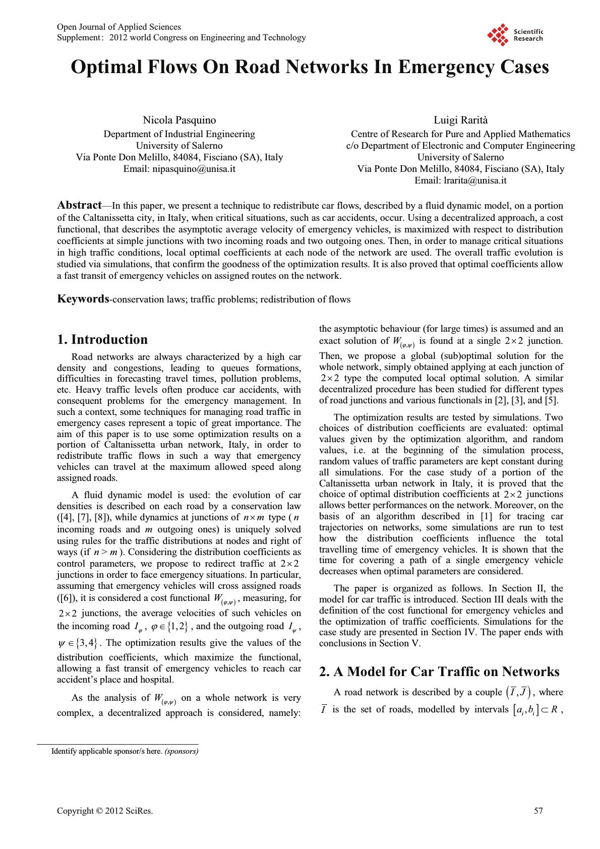Optimal Flows On Road Networks In Emergency Cases
Nicola Pasquino
Department of Industrial Engineering
University of Salerno
Via Ponte Don Melillo, 84084, Fisciano (SA), Italy
Luigi Rarità
Centre of Research for Pure and Applied Mathematics
c/o Department of Electronic and Computer Engineering
University of Salerno
Via Ponte Don Melillo, 84084, Fisciano (SA), Italy
Abstract—In this paper, we present a technique to redistribute car flows, described by a fluid dynamic model, on a portion
of the Caltanissetta city, in Italy, when critical situations, such as car accidents, occur. Using a decentralized approach, a cost
functional, that describes the asymptotic average velocity of emergency vehicles, is maximized with respect to distribution
coefficients at simple junctions with two incoming roads and two outgoing ones. Then, in order to manage critical situations
in high traffic conditions, local optimal coefficients at each node of the network are used. The overall traffic evolution is
studied via simulations, that confirm the goodness of the optimization results. It is also proved that optimal coefficients allow
a fast transit of emergency vehicles on assigned routes on the network.
Keywords-conservation laws; traffic problems; redistribution of flows
1.Introduction
Road networks are always characterized by a high car
density and congestions, leading to queues formations,
difficulties in forecasting travel times, pollution problems,
etc. Heavy traffic levels often produce car accidents, with
consequent problems for the emergency management. In
such a context, some techniques for managing road traffic in
emergency cases represent a topic of great importance. The
aim of this paper is to use some optimization results on a
portion of Caltanissetta urban network, Italy, in order to
redistribute traffic flows in such a way that emergency
vehicles can travel at the maximum allowed speed along
assigned roads.
A fluid dynamic model is used: the evolution of car
densities is described on each road by a conservation law
([4], [7], [8]), while dynamics at junctions of nmu type ( n
incoming roads and m
outgoing ones) is uniquely solved
using rules for the traffic distributions at nodes and right of
ways (if >nm ). Considering the distribution coefficients as
control parameters, we propose to redirect traffic at 22u
junctions in order to face emergency situations. In particular,
assuming that emergency vehicles will cross assigned roads
([6]), it is considered a cost functional

,
W
M\
, measuring, for
22u
junctions, the average velocities of such vehicles on
the incoming road I
M
,
^`
1,2 M  , and the outgoing road I
\
,
^`
3,4
\

. The optimization results give the values of the
distribution coefficients, which maximize the functional,
allowing a fast transit of emergency vehicles to reach car
accident’s place and hospital.
As the analysis of

,
W
M\
on a whole network is very
complex, a decentralized approach is considered, namely:
the asymptotic behaviour (for large times) is assumed and an
exact solution of

,
W
M\
is found at a single
22u
junction.
Then, we propose a global (sub)optimal solution for the
whole network, simply obtained applying at each junction of
22u
type the computed local optimal solution. A similar
decentralized procedure has been studied for different types
of road junctions and various functionals in [2], [3], and [5].
The optimization results are tested by simulations. Two
choices of distribution coefficients are evaluated: optimal
values given by the optimization algorithm, and random
values, i.e. at the beginning of the simulation process,
random values of traffic parameters are kept constant during
all simulations. For the case study of a portion of the
Caltanissetta urban network in Italy, it is proved that the
choice of optimal distribution coefficients at 22u junctions
allows better performances on the network. Moreover, on the
basis of an algorithm described in [1] for tracing car
trajectories on networks, some simulations are run to test
how the distribution coefficients influence the total
travelling time of emergency vehicles. It is shown that the
time for covering a path of a single emergency vehicle
decreases when optimal parameters are considered.
The paper is organized as follows. In Section II, the
model for car traffic is introduced. Section III deals with the
definition of the cost functional for emergency vehicles and
the optimization of traffic coefficients. Simulations for the
case study are presented in Section IV. The paper ends with
conclusions in Section V.
2. A Model for Car Traffic on Networks
A road network is described by a couple

,IJ , where
I
is the set of roads, modelled by intervals
>@
,
ii
ab R ,
Identify applicable sponsor/s here. (sponsors)
Open Journal of Applied Sciences
Supplement：2012 world Congress on Engineering and Technology
Cop
y
ri
g
ht © 2012 SciRes.57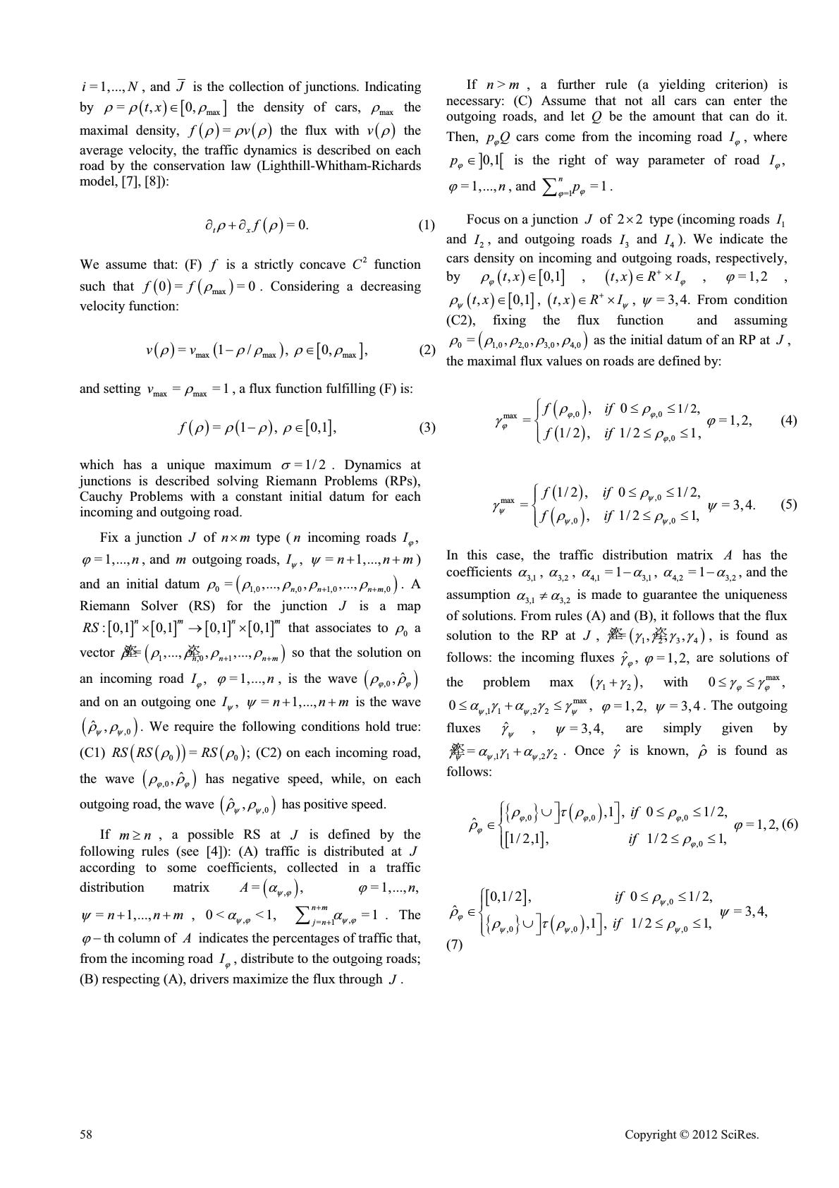

= 1,...,iN
, and
J
is the collection of junctions. Indicating
by
 >@
max
=, 0,tx UU U 
the density of cars,
max
U
the
maximal density,

=fv UUU
the flux with

v U
the
average velocity, the traffic dynamics is described on each
road by the conservation law (Lighthill-Whitham-Richards
model, [7], [8]):

=0.
tx
f UU ww (1)
We assume that: (F) f is a strictly concave
2
C function
such that
 
max
0= =0ff U . Considering a decreasing
velocity function:
  >@
max maxmax
=1/, 0,,vv U UUUU  (2)
and setting
max max
==1v U
, a flux function fulfilling (F) is:
  >@
=1, 0,1,f UU UU  (3)
which has a unique maximum =1/2 V
. Dynamics at
junctions is described solving Riemann Problems (RPs),
Cauchy Problems with a constant initial datum for each
incoming and outgoing road.
Fix a junction J of nmu type ( n incoming roads ,I
M
= 1,...,n M
, and m outgoing roads, ,I
\
= 1,...,nnm
\

)
and an initial datum

01,0,0 1,0,0
=,..., ,,...,
nn nm
UU UUU

. A
Riemann Solver (RS) for the junction J is a map
>@>@ >@>@
:0,1 0,10,1 0,1
nm nm
RS uou
that associates to
0
U
a
vector

1,01
වව"= ,...,,,...,
nn nm
UU UUU

so that the solution on
an incoming road ,I
M
= 1,...,n M , is the wave

,0
ˆ
,
MM
UU
and on an outgoing one ,I
\
= 1,...,nnm
\

is the wave

,0
ˆ,
\\
UU . We require the following conditions hold true:
(C1)
  
00
=;RS RSRS UU (C2) on each incoming road,
the wave

,0
ˆ
,
MM
UU has negative speed, while, on each
outgoing road, the wave

,0
ˆ,
\\
UU has positive speed.
If mnt, a possible RS at J
is defined by the
following rules (see [4]): (A) traffic is distributed at J
according to some coefficients, collected in a traffic
distribution matrix

,
=,A
\M
D = 1,...,,n M
= 1,...,nnm
\

,
,
0< <1,
\M
D
,
=1
=1
nm
jn
\M
D


¦
. The
M 
th column of A indicates the percentages of traffic that,
from the incoming road I
M
, distribute to the outgoing roads;
(B) respecting (A), drivers maximize the flux through J
.
If >nm , a further rule (a yielding criterion) is
necessary: (C) Assume that not all cars can enter the
outgoing roads, and let Q
be the amount that can do it.
Then, pQ
M
cars come from the incoming road I
M
, where
@>
0,1p
M

is the right of way parameter of road
,I
M
= 1,...,n M
, and
=1
=1
n
p
M
M
¦
.
Focus on a junction J of 22u type (incoming roads
1
I
and
2
I
, and outgoing roads
3
I
and
4
I
). We indicate the
cars density on incoming and outgoing roads, respectively,
by
 >@
,0,1tx
M
U  ,

,txR I
M

u , =1,2 M ,
 >@
,0,1tx
\
U 
,

,txR I
\

u
,
=3,4.
\
From condition
(C2), fixing the flux function and assuming

01,0 2,03,0 4,0
=,,, UUUUU
as the initial datum of an RP at
J
,
the maximal flux values on roads are defined by:


,0 ,0
max
,0
1/2 , 0,
= =1,2,
1/2, 1/21,
fif
fif
MM
M
M
UU
JM
U
dd
°
®dd
°
¯
(4)


,0
max
,0 ,0
1/2, 01/2,
= =3,4.
, 1/21,
fif
fif
\
\
\\
U
J\
UU
dd 
°
®dd
°
¯
(5)
In this case, the traffic distribution matrix A has the
coefficients
3,1
D
,
3,2
D
,
4,13,1
=1 DD 
,
4,2 3,2
=1 DD 
, and the
assumption
3,1 3,2
DD z is made to guarantee the uniqueness
of solutions. From rules (A) and (B), it follows that the flux
solution to the RP at J ,

1234
වව"=,,,
JJJJJ , is found as
follows: the incoming fluxes
ˆ
M
J , =1,2, M are solutions of
the problem max

12
, JJ 
with
max
0,
MM
JJ dd
max
,1 1,22
0,
\\ \
DJ DJJ d d =1,2, M =3,4
\
. The outgoing
fluxes
ˆ
\
J
,
=3,4,
\
are simply given by
,1 1,22
ව"=
\\ \
JDJDJ  . Once ˆ
J
is known, ˆ
U
is found as
follows:
^` 
>@
,0 ,0,0
,0
,1, 01/2,
ˆ =1,2,
1/2,1, 1/21,
if
if
MM M
M
M
UWUU
UM
U
ºº
dd
°¼¼
®dd
°
¯
(6)
>@
^` 
,0
,0 ,0,0
0,1/2, 01/2,
ˆ =3,4,
,1, 1/21,
if
if
\
M
\\ \
U
U\
UWU U
dd
°
®ºº
dd
°¼¼
¯
(7)
58 Cop
y
ri
g
ht © 2012 SciRes.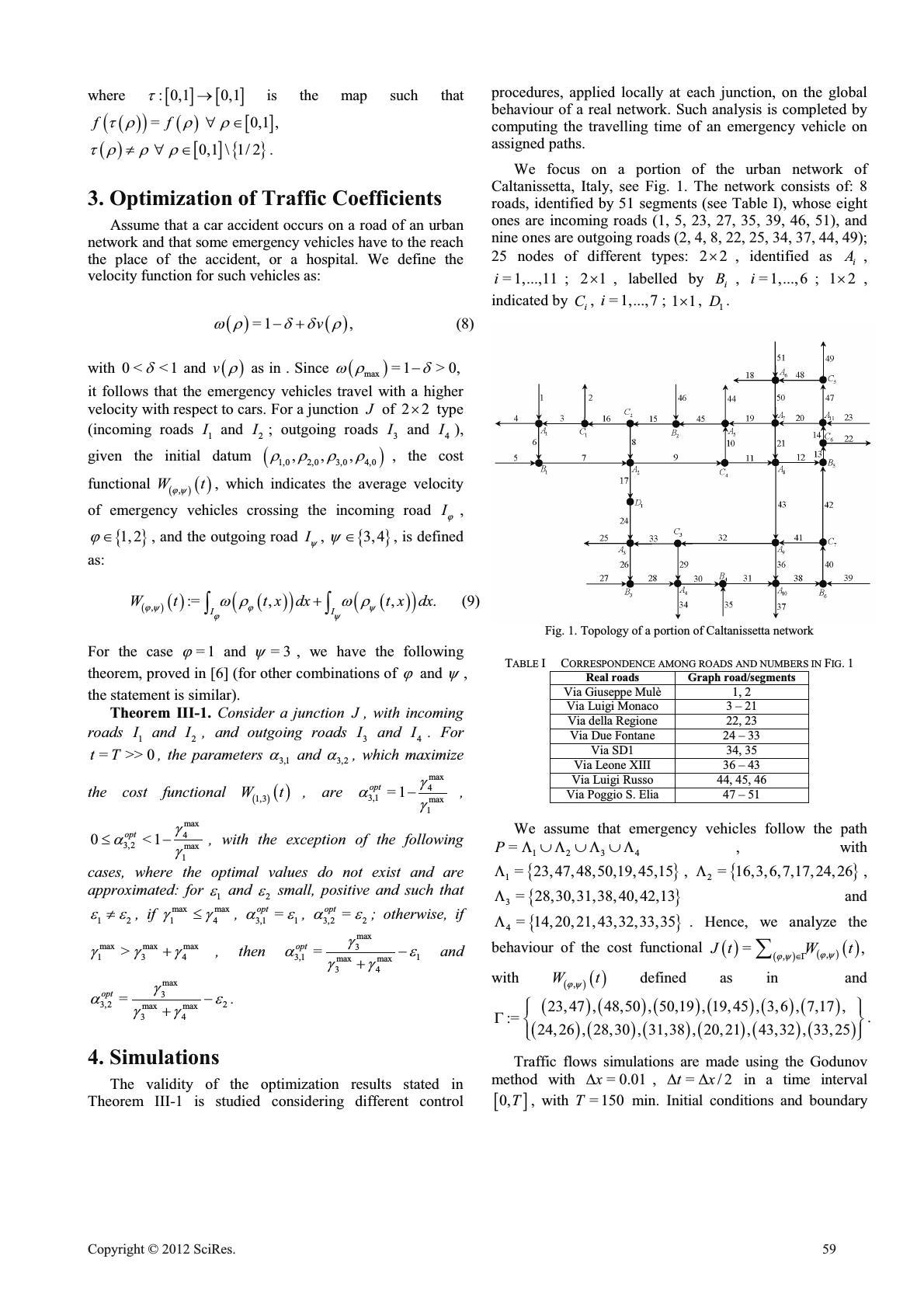

where
>@>@
: 0,10,1 W o is the map such that
   >@
= 0,1,ff WUU U 
 >@ ^`
0,1\1/2 WUUU z
.
3. Optimization of Traffic Coefficients
Assume that a car accident occurs on a road of an urban
network and that some emergency vehicles have to the reach
the place of the accident, or a hospital. We define the
velocity function for such vehicles as:

=1 ,v ZUGGU  (8)
with 0< <1 G and

v U as in . Since

max
=1 >0, ZU G 
it follows that the emergency vehicles travel with a higher
velocity with respect to cars. For a junction J
of
22u
type
(incoming roads 1 I and
2
I ; outgoing roads
3
I and
4
I ),
given the initial datum

1,0 2,0 3,0 4,0
,,, UUUU , the cost
functional


,
Wt
M\
, which indicates the average velocity
of emergency vehicles crossing the incoming road I
M
,
^`
1,2 M 
, and the outgoing road
I
\
,
^`
3,4 \ , is defined
as:

  


,
:=,, .
II
Wttx dxtx dx
M\
M\ M\
ZU ZU 
³³
(9)
For the case
=1 M
and
=3
\
, we have the following
theorem, proved in [6] (for other combinations of M
and
\
,
the statement is similar).
Theorem III-1. Consider a junction J
, with incoming
roads
1
I and
2
I , and outgoing roads
3
Iand
4
I . For
=>>0tT , the parameters
3,1
D and
3,2
D , which maximize
the cost functional


1,3
Wt
, are
max
4
3,1 max
1
=1
opt
J
DJ 
,
max
4
3,2 max
1
0<1
opt
J
DJ
d
, with the exception of the following
cases, where the optimal values do not exist and are
approximated: for
1
H and
2
H small, positive and such that
12
HH z, if
max max
14
JJ d
,
3,1 1
=
opt
DH ,3,2 2 =
opt
DH ; otherwise, if
maxmax max
134
> JJJ 
, then
max
3
3,1 1
max max
34
=
opt
J
DH
JJ


and
max
3
3,2 2
max max
34
=
opt
J
DH
JJ


.
4. Simulations
The validity of the optimization results stated in
Theorem III-1 is studied considering different control
procedures, applied locally at each junction, on the global
behaviour of a real network. Such analysis is completed by
computing the travelling time of an emergency vehicle on
assigned paths.
We focus on a portion of the urban network of
Caltanissetta, Italy, see Fig. 1. The network consists of: 8
roads, identified by 51 segments (see Table I), whose eight
ones are incoming roads (1, 5, 23, 27, 35, 39, 46, 51), and
nine ones are outgoing roads (2, 4, 8, 22, 25, 34, 37, 44, 49);
25 nodes of different types: 22u , identified as
i
A,
= 1,...,11i ; 21u , labelled by
i
B, = 1,...,6i ; 12u ,
indicated by
i
C, = 1,...,7i
;
11u
,
1
D
.
Fig. 1. Topology of a portion of Caltanissetta network
TABLE I CORRESPONDENCE AMONG ROADS AND NUMBERS IN FIG. 1
Real roadsGraph road/segments
Via Giuseppe Mulè 1, 2
Via Luigi Monaco 3 – 21
Via della Regione 22, 23
Via Due Fontane 24 – 33
Via SD1 34, 35
Via Leone XIII 36 – 43
Via Luigi Russo 44, 45, 46
Via Poggio S. Elia 47 – 51
We assume that emergency vehicles follow the path
1234
=P//// , with
^`
1
= 23,47,48,50,19,45,15/
,
^`
2
= 16,3,6,7,17,24,26/
,
^`
3= 28,30,31,38,40,42,13/
and
^`
4= 14,20,21,43,32,33,35/
. Hence, we analyze the
behaviour of the cost functional

 

,
,
=,JtW t
M\
M\ *
¦
with


,
Wt
M\
defined as in and


23,47 ,48,50, 50,19 ,19,45, 3,6 , 7,17,
:= 24,26, 28,30, 31,38,20,21, 43,32 , 33,25
½
°°
*®¾
°°
¯¿
.
Traffic flows simulations are made using the Godunov
method with = 0.01x', =/2tx'' in a time interval
>@
0,T
, with
= 150T
min. Initial conditions and boundary
Cop
y
ri
g
ht © 2012 SciRes.59

data for densities have been chosen approaching
max
=1 U ,
with the aim of simulating a congestion scenario on the
network, and are the following: initial datum equal to 0.8 for
all roads; boundary data 0.9 for roads 1, 5, 23, 27 and 35;
0.95 for roads 39, 46, and 51; 0.8 for roads 2, 4, 18, 22 and
25; 0.85 for roads 34, 37, 44 and 49. According to measures
on the real network, we set, for junctions i B, = 1,...,6i
, the
following right of way parameters:
12 26
== 0.2pp ,
46
= 0.3p
,
635
== 0.4pp
, 38 39
==0.5pp ,
530
==0.6pp
,
45
= 0.7p
, 42 27
== 0.8pp ; for junctions i C,
= 1,...,7i , the
following distribution coefficients:
49,47 22,13
== 0.3 DD
,
8,1533,32
==0.4 DD
,
41,40 = 0.2
D
,
2,16 3,16 10,9 11,9
====0 DDDD
,
42,40 = 0.8
D
,
16,1529,32
== 0.6 DD
,
48.47 14,13
== 0.7 DD
. Moreover,
= 0.5 G is considered.
We analyze two different simulation cases: locally
optimal distribution coefficients (optimal case) at each
junction
i
A, = 1,...,11i , i. e. parameters according to
Theorem III-1; random parameters (random case), namely
the distribution coefficients are taken randomly for each
junction
i
A, = 1,...,11i , when the simulation starts and then
are kept constant.
In Fig. 2, the behaviour of the cost functional

Jt is
represented. The optimal simulation is indicated by a
continuous line, while random cases by dashed curves. As
expected, random simulations lines of

Jt are always
lower than the optimal one. In fact, when optimal parameters
are used, junctions of 22u type are interested by a
congestion reduction, due to the flows redistribution on
roads. Even if right of way parameters of junctions i B,
= 1,...,6i
, and distribution coefficients of junctions i
C,
= 1,...,7i
, are optimized using the results in [2] and [3],
traffic conditions are almost unaffected.
Suppose that an emergency vehicle travels along a path
in a network. Its position

=xxt
is obtained solving the
Cauchy problem:
 

00
=,,
=,
xtx
xt x
ZU

°
®
°
¯
 (10)
where
0
x is the initial position at the initial time 0 t. Using
numerical methods, described in [1], it is possible to
estimate the travelling time of the emergency vehicle. First,
we compute the trajectory along road 45 and the time
needed for covering it in optimal case and random cases;
then, we consider the path P and study the exit time
evolution versus the initial travel time 0 t (the time in which
the emergency vehicle enters into the network).
Fig. 2. Evolution of ()Jt in
>@
0,60 using optimal distribution coefficients
(continuous line) and random choices (dashed lines)
In Fig. 3, we assume that the emergency vehicle starts
its own travel at the beginning of road 45 at the initial time
0=40t
and compute the trajectories ()xt along road 45, in
optimal (continuous line) and random cases (dashed lines).
Fig. 3. Trajectory ()xt for an emergency vehicle along road 45 with
0
=40,t
optimal coefficients (continuous line) and random choices
(dashed lines)
The evolution ()xt in the optimal case has always a
higher slope with respect to trajectories in random cases
because traffic levels are low. When random distribution
coefficients are used, shocks propagating backwards
increase the density values on the whole network; the
velocity for the emergency vehicles is reduced and exit
times from road 45 become longer. In Table II, assuming
0=40t
we report the time instants
out
t
in which the
emergency vehicle goes out of road 45, either for the
optimal values of distribution coefficients (opt) or random
choices (i r, = 1,..,4i ).
TABLE II. TIMES
out
t , ASSUMING
0
=40t
Simulationsopt
1
r
2
r
3
r
4
r
out
t 45.70 51.34 49.94 47.84 46.42
60 Cop
y
ri
g
ht © 2012 SciRes.

The exit time 00 ()=
exit out
Tt t t from road 45 versus the
initial time 0 t, assuming that the emergency vehicle starts
its path from the beginning of the road, is depicted in Fig. 4.
Notice that the choice of optimal coefficients (continuous
line) allows to obtain an exit time lower than the other cases
(dashed lines), due to decongestion effects. The exit time
becomes stable after a certain initial time value (
0
9.45t
for the optimal distribution choice, unlike the random cases,
for which
05.1t
, 05.3t , 06.3t and 07.4t ).
In Fig. 5, we report the exit time
0
()
exit
Tt from the
chosen path P versus the initial times
0
t. When optimal
parameters are not used,
0
()
exit
Tt
is the lowest curve, as
expected, because the network is not congested.
Furthermore,
0
()
exit
Tt never tends to infinity as the
emergency vehicle has a higher velocity with respect to cars,
hence it is able to reach its own destination although some
roads of the chosen path are completely blocked. The steady
value of
0
()
exit
Tt is reached at time
0
6.9t .
Fig. 4. Exit time from road 45 vs
0
t in
>@
0,30 ; optimal coefficients
(continuous line) and random choices (dashed lines).
Fig. 5. Exit time from the path P vs
0
t
in
>@
0,40
; optimal coefficients
(continuous line) and random choices (dashed lines)
5. Conclusions
In this paper, it is presented an optimization study to
manage emergency situations on road networks. Optimal
distribution coefficients at road junctions with two
incoming roads and two outgoing ones have been computed
maximizing a cost functional, that measures the average
velocity of emergency vehicles. Simulations have been
made on a real urban network. It has been proved, through a
numerical evaluation of emergency vehicles trajectories,
that fast transits are possible also in cases of high
congestions.
REFERENCES
[1] G. Bretti, and B. Piccoli, “A tracking algorithm for car
paths on road networks,” SIAM Journal on Applied
Dynamical Systems, vol. 7, pp. 510–531, 2008.
[2] A. Cascone, C. D’Apice, B. Piccoli, and L. Rarità,
“Optimization of traffic on road networks,”
Mathematical Models and Methods in Applied
Sciences, vol. 17, no. 10, pp. 1587–1617, 2007.
[3] A. Cascone, C. D’Apice, B. Piccoli, and L. Rarità,
“Circulation of car traffic in congested urban areas,”
Communication in Mathematical Sciences, vol. 6, no. 3,
pp. 765–784, 2008.
[4] G. Coclite, M. Garavello, and B. Piccoli, “Traffic Flow
on Road Networks,” SIAM Journal on Mathematical
Analysis, vol. 36, no. 6, pp. 1862–1886, 2005.
[5] C. D’Apice, R. Manzo, and L. Rarità, “Splitting of
Traffic Flows to Control Congestion in Special
Events,” International Journal of Mathematics and
Mathematical Sciences, vol. 2011, pp. 1–18, 2011,
Article ID 563171, doi:10.1155/2011/563171.
[6] R. Manzo, B. Piccoli, and L. Rarità, “Optimal
distribution of traffic flows at junctions in emergency
cases,” European Journal of Applied Analysis, vol. 23,
no. 4, pp. 515–535, 2012.
[7] M. J. Lighthill, and G. B. Whitham, “On kinetic waves.
II. Theory of Traffic Flows on Long Crowded Roads,”
Proc. Roy. Soc. London Ser. A, vol. 229, pp. 317–345,
1955.
[8] P. I. Richards, “Shock Waves on the Highway,” Oper.
Res., vol. 4, pp. 42–51, 1956.
Cop
y
ri
g
ht © 2012 SciRes.61