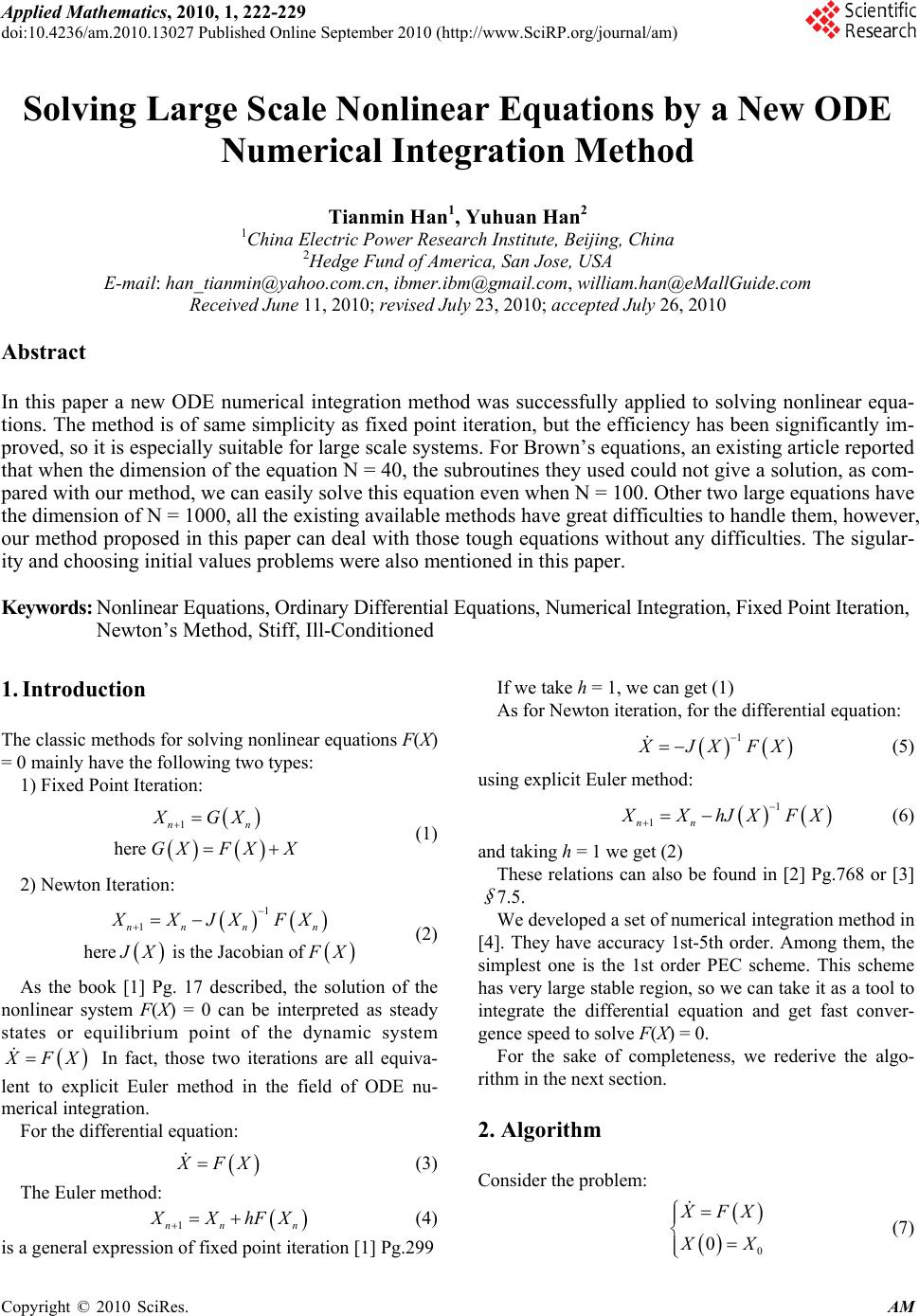Applied Mathematics, 2010, 1, 222-229
doi:10.4236/am.2010.13027 Published Online September 2010 (http://www.SciRP.org/journal/am)
Solving Large Scale Nonlinear Equations by a New ODE
Numerical Integration Method
Tianmin Han1, Yuhuan Han2
1China Electric Power Research Institute, Beijing, China
2Hedge Fund of America, San Jose, USA
Received June 11, 2010; revised July 23, 2010; accepted July 26, 2010
Abstract
In this paper a new ODE numerical integration method was successfully applied to solving nonlinear equa-
tions. The method is of same simplicity as fixed point iteration, but the efficiency has been significantly im-
proved, so it is especially suitable for large scale systems. For Brown’s equations, an existing article reported
that when the dimension of the equation N = 40, the subroutines they used could not give a solution, as com-
pared with our method, we can easily solve this equation even when N = 100. Other two large equations have
the dimension of N = 1000, all the existing available methods have great difficulties to handle them, however,
our method proposed in this paper can deal with those tough equations without any difficulties. The sigular-
ity and choosing initial values problems were also mentioned in this paper.
Keywords: Nonlinear Equations, Ordinary Differential Equations, Numerical Integration, Fixed Point Iteration,
Newton’s Method, Stiff, Ill-Conditioned
1. Introduction
The classic methods for solving nonlinear equations F(X)
= 0 mainly have the following two types:
1) Fixed Point Iteration:

 
1
here
nn
XGX
GXFX X


(1)
2) Newton Iteration:
 
 
1
1
here is the Jacobian of
nn nn
XXJXFX
J
XFX

 (2)
As the book [1] Pg. 17 described, the solution of the
nonlinear system F(X) = 0 can be interpreted as steady
states or equilibrium point of the dynamic system

X
FX
 In fact, those two iterations are all equiva-
lent to explicit Euler method in the field of ODE nu-
merical integration.
For the differential equation:


X
FX
 (3)
The Euler method:


1nn n
X
XhFX
 (4)
is a general expression of fixed point iteration [1] Pg.299
If we take h = 1, we can get (1)
As for Newton iteration, for the differential equation:
 
1
X
JX FX


 (5)
using explicit Euler method:
 
1
1nn
X
XhJXFX

 (6)
and taking h = 1 we get (2)
These relations can also be found in [2] Pg.768 or [3]
§ 7.5.
We developed a set of numerical integration method in
[4]. They have accuracy 1st-5th order. Among them, the
simplest one is the 1st order PEC scheme. This scheme
has very large stable region, so we can take it as a tool to
integrate the differential equation and get fast conver-
gence speed to solve F(X) = 0.
For the sake of completeness, we rederive the algo-
rithm in the next section.
2. Algorithm
Consider the problem:


0
0
X
FX
X
X






(7)

T. M. HAN ET AL.
223
Using implicit Euler method:

11nn n
XXhFX

 (8)
introducing variable


11nn
ZhFX

 (9)
we have
11nnn
Z
XX

 (10)
Multiplying both sides of (9) by

(

> 0), we ob-
tain

11nn
ZhFX 

 (11)
Equation (11) can be reformulated as follows:
 
11nn
hZF X 

 (12)
Equation (12) plus Equation (10), we obtain



111
1nnnn hZF XXX 

  (13)
Let

hh

  (14)
Equation (13) can be rewritten as
 
111nnnn
Z
FXX X 

 (15)
From (8) and (9), we have
11nnn
X
XZ

 (16)
Combining (15) and (16), we obtain a new implicit in-
tegration method, which is fully equivalent to (8).
We use the simple iteration method to solve the im-
plicit system (15) and (16), and choose the initial itera-
tion value


0
1 nnn
X
XZ
. Only one iteration applies to
the implicit system (15) and (16), then we obtain an ex-
plicit integration scheme as follows:


 
0
1
0
11
11
nnn
nnn
nnn
XXZ
Z
FX Z
XXZ











(17)
(17) is named as the EPS method in this article.
In order to investigate the stability of the EPS method
(17), we consider the model equation
x
x


 (18)
where

is a complex number. Then, we have

11
1
nnn
nnnn
xxz
zxzz

 







 (19)
or the matrix form
1
1
1
nn
nn
x
x
zz
 
 



  

 



 
(20)
The characteristic equation of (20) is given by


2121 0


 (21)
Let
h



(22)
From (21), we obtain



21
21
h

 



 (23)
Giving

a special value, let

vary and keep


1,
then we obtain an enclosed curve, which is just the
boundary of the absolute stability region in h

-plane.
Set cos sinj



, 1j

, 02

  , then we
rewrite (23) as follows:




 

 
2
2
Re12sincoscos
12cos22 cos1sin54 cos
h 

 
 
 
(24)




   
2
Im212sincoscossin
2cos1sin1 2cos54cos
h



 


(25)
The curve of the boundary of the absolute stability re-
gion is obtained when

varies from 0 to 2

. If

is
a small number, the stability region will be close to real
axis and spreads far away towards the left-half plane. For
example, when

= 0.01, as it is shown in Figure 1, the
left end point of the stability region can reach −134, so
the integration step size can be increased significantly.
Figure 1. The absolute stability region of the EPS method
for α = 0.01.

T. M. HAN ET AL.
224
In the model Equation (18), if

is very close to the
imaginary axis, i.e.,
 
Im Re

 ,

should be taken
a bigger value. For

= 100, the stability region is
shown by Figure 4. We can find that the region includes
a section of the imaginary axis. This property is unusual
for an explicit method.
When

= 1, i.e., h =

, then the stability region of
the EPS method is all the same as the explicit Euler
method. It is enclosed by a circle with center at (−1, 0)
and its radius is 1. In fact, in (24) and (25) taking α = 1,
then

= 0.5, we have
Figure 2. The absolute stability region of the EPS method
for α = 0.1.
Figure 3. The absolute stability region of the EPS method
for α = 10.
Figure 4. The absolute stability region of the EPS method
for α = 100.







2
22
Re1.52sin1.5cos1 2cos
4cossin3sin2.52cos
cos1
h

 

 

 
 

(26)




 

2
2
Im34 sin3cossin
5cos1.5 4cossin2.52cos
sin
h 

 

 
 

(27)
3. Implementation of the Algorithm
In this article, we merely discuss how to use the EPS
method to integrate the differential equation


X
FX
.
Usually ODE integration methods require the condition
0FX

 holds. That is to say the eigenvalues of the
Jacobian distribute in the left-half part of the complex
plane. For our purpose, to solve F(x) = 0 and to solve
−F(x) = 0 are equivalent. In other field the “half plane
condition” is always said to be “positive definite”, i.e.,
the eigenvalues are in the right plane. This fact reminds
us the differential equation to deal with is


X
FX
.
The EPS method can also be applied to the differential
equation
 
1
X
JX FX


 (28)
In this case, if F(X) is replaced with −F(X) in (28), it
does not change the form of (28). So the sign in front of
F(X) is meaningless at all. By the way, choosing ε = h =
1, according to many numerical experiments have done
by us, the numerical results of EPS are almost the same

T. M. HAN ET AL.
225
as the numerical results of the Newton’s method (the
details are not given in this article).
Despite the EPS method is a Jacobian-Free method, if
it is not difficult to obtain the diagonal matrix D(X) of
the Jacobian J(X), then we can integrate differential
equation
 
1
X
DX FXGX

 

we can get even much better results, especially, when
J(X) is a diagonal dominant matrix. However, it needs to
consider a strategy to avoid overflow when some ele-
ments of the matrix D(X) are very small.
At present we have not developed a adaptive program
which can automatically choose parameter ε and the step
size h, but we give a strategy roughly as follows.
For non-stiff system, we pick up the parameter ε on
[0.5, 1.0] and determine h by the size of

F
X. For
stiff system, we need to estimate the spectral radius ρ of
the Jacobian matrix J(X) such that

< 1 is satisfied.
In fact, if

is a positive real number, for
x
x



,
when 43

 , we can prove that the scheme (19) is
stable for all h (0h). Small value ε can strengthen
stability but will reduce the efficiency.
For some easy problems we can take fixed step size in
the whole calculating process. Usually we divide the
calculating process into three stages, in each stage, dif-
ferent step size will be taken.
To do this, we set three parameters TOL1, TOL2, TOL3.
At first, we choose step size h1 to start the calculation till
F
< TOL1 is satisfied, the first stage is completed.
Taking current value of X as initial value, we start the
second stage calculation with step size h2 till
F
< TOL2.
Do the same as we have done till finally
F
< TOL3,
then we end our calculation. In this paper, the .
means Euclidean norm.
Outline of the Algorithm
Step 1. Give an initial value 0
X
. Set

, h and com-
pute

hh

  .
Step 2. Compute

F
X and

DX if it is needed.
Step 3. Compute
 
1
GXDX FX

 or


GX


F
X. If an element

i
dX
of matrix

DX is less
than one, the division is omitted and we have


i
gX


i
f
X.
Step 4. Compute


00
Z
hG X.
Step 5. :
X
XZ.
Step 6. Compute


F
X,


DX ,

GX by the way
of Step 2 and Step 3.
Step 7. If

F
XTOL, then stop, else do
 
:
:
:
XXZ
Z
GX Z
X
XZ




Go to Step 5.
4. Numerical Experiments
We now present numerical results for five examples.
Some of them have already had results in literature. So
we can compare our results with theirs. We also compare
the results of fixed point iteration (explicit Euler method)
with ours as well. This is because we identify our method
as an improvement for the fixed point iteration and the
explicit Euler method was well represented in all explicit
methods.
4.1. Example 1 [2]


2
112
1fXx x



21 2
cos 2
f
Xx x


 

The initial value x0 = (1, 0). The solution we want to
seek is x* = (0, 1). The Jacobian of the system is:

1
2
21
1sin
22
x
JX x















and the determinant of the Jacobian is given by
 
12
detsin 1
2
JX xx







So at the line 2
1
1
sin 2x
x





 , the singularity oc-
curs.
Newton method does not converge to
x
 but rather,
it crosses the singularity line and converges in eight it-
erations to 13 2,
22
x 


.
The damped Newton method was also applied to this
problem and it converged to x* in 107 iterations. The
total number of function evaluations is as many as 321.
In [2], there are 12 algorithms, all of them are based
on trapezoid formula, have been tested for this example.
Among them the PEBCEB is the best, here the EB means
using Broyden method to approximate J−1. The iteration
is 17 times and the evaluation is 36 times.
There are four algorithms, each of them needs iterate
more than 100 times. The rest seven algorithms need to
iterate 23~47 times and evaluate 68~282 times respec-
tively. All those calculations use double precision.
This example was considered as a difficult problem,
because the differential equation to deal with is
X


 
1
J
XFX

 and the Jacobian is singular.
If the differential equation to be handled is


X
FX
,
all the trouble will disappear. In fact it is a non-stiff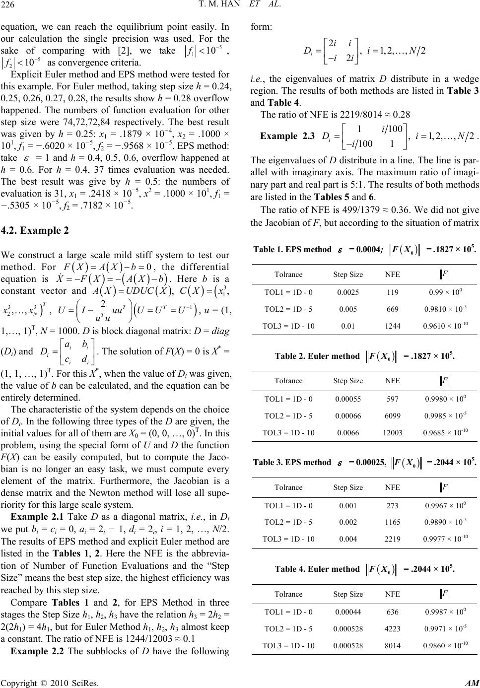

T. M. HAN ET AL.
226
equation, we can reach the equilibrium point easily. In
our calculation the single precision was used. For the
sake of comparing with [2], we take 5
110f

,
5
210f
 as convergence criteria.
Explicit Euler method and EPS method were tested for
this example. For Euler method, taking step size h = 0.24,
0.25, 0.26, 0.27, 0.28, the results show h = 0.28 overflow
happened. The numbers of function evaluation for other
step size were 74,72,72,84 respectively. The best result
was given by h = 0.25: x1 = .1879 × 10−4, x2 = .1000 ×
101, f1 = −.6020 × 10−5, f2 = −.9568 × 10−5. EPS method:
take

= 1 and h = 0.4, 0.5, 0.6, overflow happened at
h = 0.6. For h = 0.4, 37 times evaluation was needed.
The best result was give by h = 0.5: the numbers of
evaluation is 31, x1 = .2418 × 10−5, x2 = .1000 × 101, f1 =
−.5305 × 10 −5, f2 = .7182 × 10−5.
4.2. Example 2
We construct a large scale mild stiff system to test our
method. For
 
0FXAX b, the differential
equation is
 


X
FXAX b 
. Here b is a
constant vector and
 
A
XUDUC X,


3
1
CX x,

33
2,, T
N
xx,

1
2TT
T
UI uuUUU
uu


 

 , u = (1,
1,…, 1)T, N = 1000. D is block diagonal matrix: D = diag
(Di) and ii
i
ii
ab
Dcd



. The solution of F(X) = 0 is X* =
(1, 1, …, 1)T. For this X*, when the value of Di was given,
the value of b can be calculated, and the equation can be
entirely determined.
The characteristic of the system depends on the choice
of Di. In the following three types of the D are given, the
initial values for all of them are X0 = (0, 0, …, 0)T. In this
problem, using the special form of U and D the function
F(X) can be easily computed, but to compute the Jaco-
bian is no longer an easy task, we must compute every
element of the matrix. Furthermore, the Jacobian is a
dense matrix and the Newton method will lose all supe-
riority for this large scale system.
Example 2.1 Take D as a diagonal matrix, i.e., in Di
we put bi = ci = 0, ai = 2i − 1, di = 2i, i = 1, 2, …, N/2.
The results of EPS method and explicit Euler method are
listed in the Tables 1, 2. Here the NFE is the abbrevia-
tion of Number of Function Evaluations and the “Step
Size” means the best step size, the highest efficiency was
reached by this step size.
Compare Tables 1 and 2, for EPS Method in three
stages the Step Size h1, h2, h3 have the relation h3 = 2h2 =
2(2h1) = 4h1, but for Euler Method h1, h2, h3 almost keep
a constant. The ratio of NFE is 1244/12003 ≈ 0.1
Example 2.2 The subblocks of D have the following
form:
2,1,2,,2
2
i
ii
DiN
ii






i.e., the eigenvalues of matrix D distribute in a wedge
region. The results of both methods are listed in Table 3
and Table 4.
The ratio of NFE is 2219/8014 ≈ 0.28
Example 2.3 1100
,1,2,,2
100 1
i
i
DiN
i





.
The eigenvalues of D distribute in a line. The line is par-
allel with imaginary axis. The maximum ratio of imagi-
nary part and real part is 5:1. The results of both methods
are listed in the Tables 5 and 6.
The ratio of NFE is 499/1379 ≈ 0.36. We did not give
the Jacobian of F, but according to the situation of matrix
Table 1. EPS method

= 0.0004; 
0
FX = .1827 × 105.
Tolrance Step Size NFE
F
TOL1 = 1D - 0 0.0025 119 0.99 × 100
TOL2 = 1D - 5 0.005 669 0.9810 × 10-5
TOL3 = 1D - 10 0.01 1244 0.9610 × 10-10
Table 2. Euler method

0
FX = .1827 × 105.
Tolrance Step Size NFE
F
TOL1 = 1D - 0 0.00055 597 0.9980 × 100
TOL2 = 1D - 5 0.00066 6099 0.9985 × 10-5
TOL3 = 1D - 10 0.0066 12003 0.9685 × 10-10
Table 3. EPS method

= 0.00025,

0
F
X = .2044 × 105.
Tolrance Step Size NFE
F
TOL1 = 1D - 0 0.001 273 0.9967 × 100
TOL2 = 1D - 5 0.002 1165 0.9890 × 10-5
TOL3 = 1D - 10 0.004 2219 0.9977 × 10-10
Table 4. Euler method

0
FX = .2044 × 105.
Tolrance Step Size NFE
F
TOL1 = 1D - 0 0.00044 636 0.9987 × 100
TOL2 = 1D - 5 0.000528 4223 0.9971 × 10-5
TOL3 = 1D - 10 0.000528 8014 0.9860 × 10-10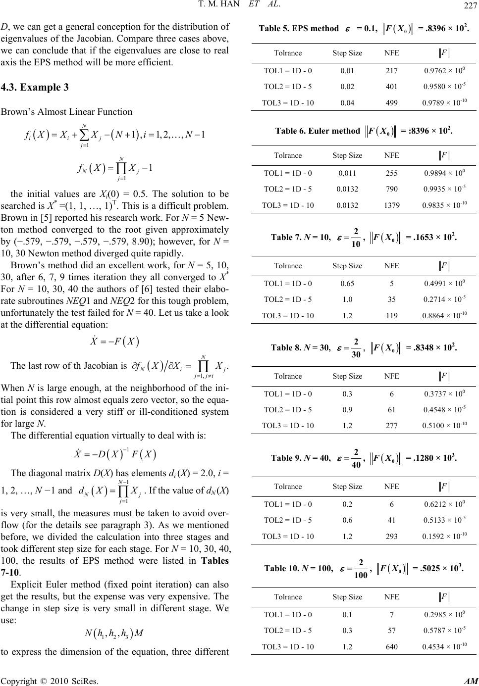

T. M. HAN ET AL.
227
D, we can get a general conception for the distribution of
eigenvalues of the Jacobian. Compare three cases above,
we can conclude that if the eigenvalues are close to real
axis the EPS method will be more efficient.
4.3. Example 3
Brown’s Almost Linear Function
 
1
1,1,2, ,1
N
iij
j
fX XXNiN

 


1
1
N
Nj
j
fX X



the initial values are Xi(0) = 0.5. The solution to be
searched is X* =(1, 1, …, 1)T. This is a difficult problem.
Brown in [5] reported his research work. For N = 5 New-
ton method converged to the root given approximately
by (−.579, −.579, −.579, −.579, 8.90); however, for N =
10, 30 Newton method diverged quite rapidly.
Brown’s method did an excellent work, for N = 5, 10,
30, after 6, 7, 9 times iteration they all converged to X*
For N = 10, 30, 40 the authors of [6] tested their elabo-
rate subroutines NEQ1 and NEQ2 for this tough problem,
unfortunately the test failed for N = 40. Let us take a look
at the differential equation:


X
FX

The last row of th Jacobian is

1,
N
N
ij
jji
f
XX X


.
When N is large enough, at the neighborhood of the ini-
tial point this row almost equals zero vector, so the equa-
tion is considered a very stiff or ill-conditioned system
for large N.
The differential equation virtually to deal with is:
 
1
X
DX FX



The diagonal matrix D(X) has elements di (X) = 2.0, i =
1, 2, …, N −1 and

1
1
N
N
j
j
dX X




. If the value of dN (X)
is very small, the measures must be taken to avoid over-
flow (for the details see paragraph 3). As we mentioned
before, we divided the calculation into three stages and
took different step size for each stage. For N = 10, 30, 40,
100, the results of EPS method were listed in Tables
7-10.
Explicit Euler method (fixed point iteration) can also
get the results, but the expense was very expensive. The
change in step size is very small in different stage. We
use:

123
,,Nhh hM
to express the dimension of the equation, three different
Table 5. EPS method

= 0.1,

0
F
X = .8396 × 102.
Tolrance Step Size NFE
F
TOL1 = 1D - 0 0.01 217 0.9762 × 100
TOL2 = 1D - 5 0.02 401 0.9580 × 10-5
TOL3 = 1D - 10 0.04 499 0.9789 × 10-10
Table 6. Euler method

0
F
X = :8396 × 102.
Tolrance Step Size NFE
F
TOL1 = 1D - 0 0.011 255 0.9894 × 100
TOL2 = 1D - 5 0.0132 790 0.9935 × 10-5
TOL3 = 1D - 10 0.0132 1379 0.9835 × 10-10
Table 7. N = 10, 2
10
 ,

0
F
X = .1653 × 102.
Tolrance Step Size NFE
F
TOL1 = 1D - 0 0.65 5 0.4991 × 100
TOL2 = 1D - 5 1.0 35 0.2714 × 10-5
TOL3 = 1D - 10 1.2 119 0.8864 × 10-10
Table 8. N = 30, 2
30
 ,

0
F
X = .8348 × 102.
Tolrance Step Size NFE
F
TOL1 = 1D - 0 0.3 6 0.3737 × 100
TOL2 = 1D - 5 0.9 61 0.4548 × 10-5
TOL3 = 1D - 10 1.2 277 0.5100 × 10-10
Table 9. N = 40, 2
40
 ,

0
F
X = .1280 × 103.
Tolrance Step Size NFE
F
TOL1 = 1D - 0 0.2 6 0.6212 × 100
TOL2 = 1D - 5 0.6 41 0.5133 × 10-5
TOL3 = 1D - 10 1.2 293 0.1592 × 10-10
Table 10. N = 100, 2
100
 ,

0
F
X = .5025 × 103.
Tolrance Step Size NFE
F
TOL1 = 1D - 0 0.1 7 0.2985 × 100
TOL2 = 1D - 5 0.3 57 0.5787 × 10-5
TOL3 = 1D - 10 1.2 640 0.4534 × 10-10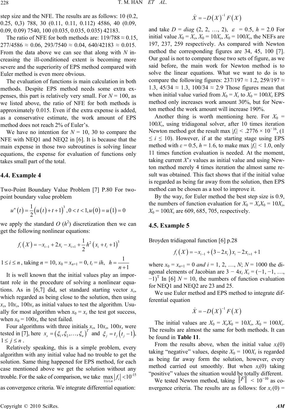

T. M. HAN ET AL.
228
step size and the NFE. The results are as follows: 10 (0.2,
0.25, 0,3) 788, 30 (0.11, 0.11, 0.112) 4586, 40 (0.09,
0.09, 0.09) 7540, 100 (0.035, 0.035, 0.035) 42183.
The ratio of NFE for both methods are: 119/788 ≈ 0.15,
277/4586 ≈ 0.06, 293/7540 ≈ 0.04, 640/42183 ≈ 0.015.
From the data above we can see that along with N in-
creasing the ill-conditioned extent is becoming more
severe and the superiority of EPS method compared with
Euler method is even more obvious.
The evaluation of functions is main calculation in both
methods. Despite EPS method needs some extra ex-
penses, this part is relatively very small. For N = 100, as
we listed above, the ratio of NFE for both methods is
approximately 0.015. Even if the extra expense is added,
as a conservative estimate, the work amount of EPS
method does not reach 2% of Euler’s.
We have no intention for N = 10, 30 to compare the
NFE with NEQ1 and NEQ2 in [6]. It is because that the
main expense in those two subroutines is solving linear
equations, the expense for evaluation of functions only
takes small part of the total.
4.4. Example 4
Two-Point Boundary Value Problem [7] P.80 For two-
point boundary value problem
 

 
3
11,01, 010
2
n
utut ttuu
we apply the standard O (h2) discretization then we can
get the following nonlinear equations:
 
3
2
11
1
21
2
iiii ii
fXxxxhxt

 
1in , taking n = 10, x0 = xn+1 = 0, ti = ih, 1
1
hn 

It is well known that the initial values play an impor-
tant role in the procedure of solving a nonlinear equa-
tions. As in [6,7] did, set standard starting vector xs,
which regarded as being close to the solution, then using
xs, 10xs, 100xs as initial values to test the algorithm. Usu-
ally for most algorithm when x0 = xs the test got success,
when x0 = 100xs the test failed.
Four algorithms with three initials xs, 10xs, 100xs were
tested in [7], here

12
,,, T
sn
x

  and


1
jjj
tt

 ,
1jn.
Relatively speaking, this is a simple problem, every
algorithm with any initial value had no trouble to get the
solution. Same thing happened for EPS method, for each
case mentioned above we get the solution without any
trouble. For the sake of comparison, we take 1 max i
in
f


10-15
as convergence criteria. We integrate differential equation:
 
1
X
DX FX



and take D = diag (2, 2, …, 2),

= 0.5, h = 2.0 For
initial value X0 = Xs, X0 = 10Xs, X0 = 100Xs, the NEFs are
197, 237, 259 respectively. As compared with Newton
method the corresponding figures are 34, 45, 100 [7].
Our goal is not to compare those two sets of figure, as we
said before, the main work for Newton method is to
solve the linear equations. What we want to do is to
compare the following figures: 237/197 ≈ 1.2, 259/197 ≈
1.3, 45/34 ≈ 1.3, 100/34 ≈ 2.9 Those figures mean that
when initial value varied from X0 = Xs to X0 = 100Xs EPS
method only increases work amount 30%, but for New-
ton method the work amount will increase 190%.
Another thing is worth mentioning here. For X0 =
100Xs, using tridiagonal solver, after 10 times iteration
Newton method got the result max |fi| < .2776 × 10−16, (1
≤ i ≤ 10). However, if at the starting stage using EPS
method with ε = 0.5, h = 1.6, to make max |fi| < 1.0, only
11 times function evaluation is needed. At the moment,
taking current X’s values as initial value and using New-
ton method merely 4 times iteration the almost same re-
sult was obtained. This fact shows that if the initial value
is regarded as being far away from the solution, then EPS
method can be chosen as a tool to improve it.
By the way, for Euler method the best step size is 0.9,
the numbers of function evaluation for X0 = XsX0 = 10Xs,
X0 = 100Xs are 609, 685, 705, respectively.
4.5. Example 5
Broyden tridiagonal function [6] p.28




11
3221
ii iii
fXxxx x


 
where x0 = xn+1 = 0 and i = 1, 2, …, N; N = 1000 the di-
agonal elements of Jacobian are 3 − 4xi Xs = (−1, −1, …,
−1)T In [6] N = 10, the numbers of function evaluation
for NEQ1 and NEQ2 are 23 and 25.
We use Euler method and EPS method to integrate dif-
ferential equation
 
1
X
DX FX



The initial values are X0 = XsX0 = 10Xs, X0 = 100Xs.
The results are almost the same for both methods. It can
be found in Table 11.
From the results above, when the initial value xi(0)
taking “negative” values, despite X0 = 100Xs is regarded
as being far away form the solution, however, every
method carried out smoothly. But when xi(0) taking
“positive” values the situation would be totally different.
We tested Newton method, taking
F
< 10−10 as co-
nvergence criteria. The results are as follows: for xi (0) =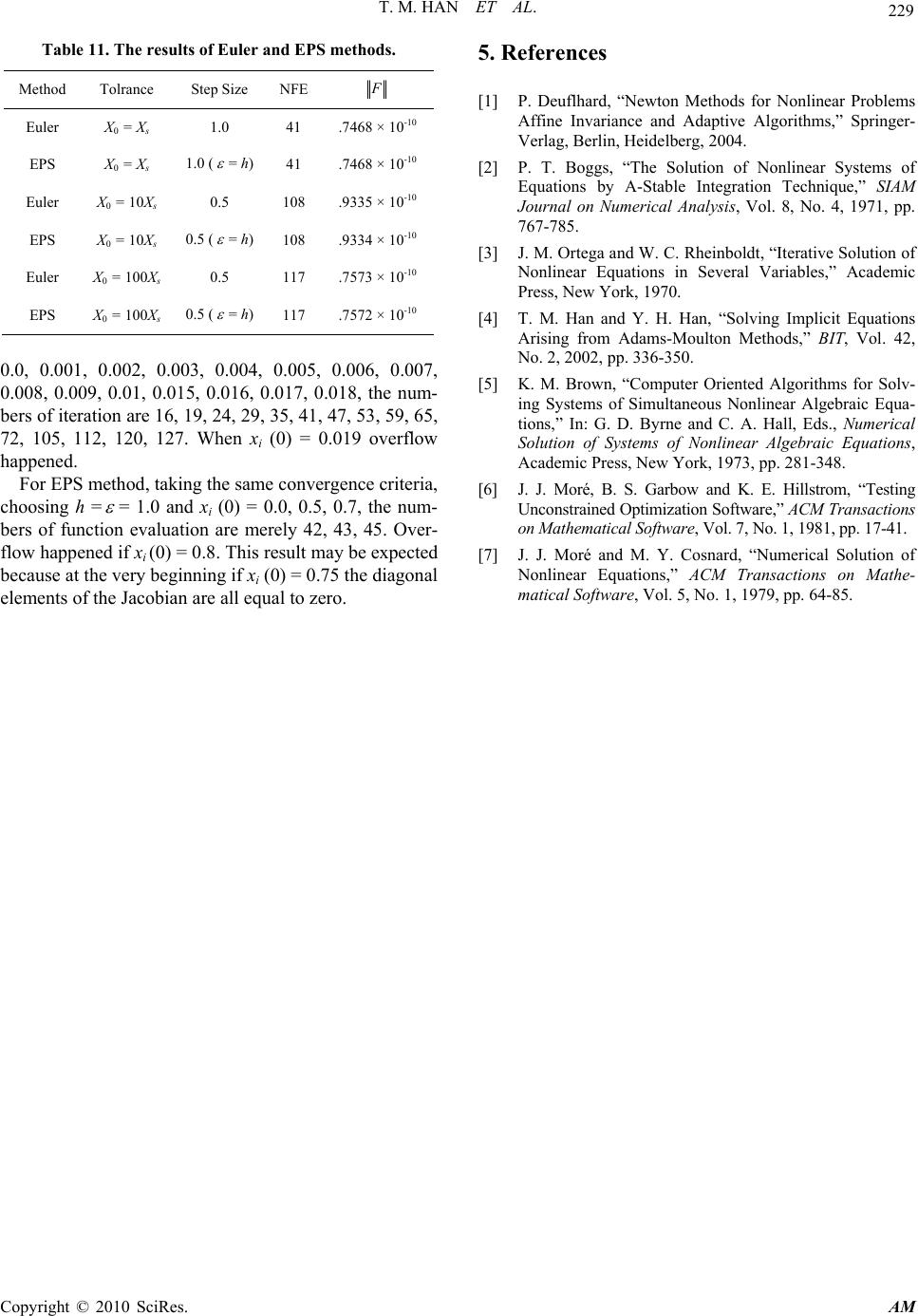

T. M. HAN ET AL.
229
Table 11. The results of Euler and EPS methods.
Method Tolrance Step Size NFE
F
Euler X0 = Xs 1.0 41 .7468 × 10-10
EPS X0 = Xs 1.0 (

= h) 41 .7468 × 10-10
Euler X0 = 10Xs 0.5 108 .9335 × 10-10
EPS X0 = 10Xs 0.5 (

= h) 108 .9334 × 10-10
Euler X0 = 100Xs 0.5 117 .7573 × 10-10
EPS X0 = 100Xs 0.5 (

= h) 117 .7572 × 10-10
0.0, 0.001, 0.002, 0.003, 0.004, 0.005, 0.006, 0.007,
0.008, 0.009, 0.01, 0.015, 0.016, 0.017, 0.018, the num-
bers of iteration are 16, 19, 24, 29, 35, 41, 47, 53, 59, 65,
72, 105, 112, 120, 127. When xi (0) = 0.019 overflow
happened.
For EPS method, taking the same convergence criteria,
choosing h =

= 1.0 and xi (0) = 0.0, 0.5, 0.7, the num-
bers of function evaluation are merely 42, 43, 45. Over-
flow happened if xi (0) = 0.8. This result may be expected
because at the very beginning if xi (0) = 0.75 the diagonal
elements of the Jacobian are all equal to zero.
5. References
[1] P. Deuflhard, “Newton Methods for Nonlinear Problems
Affine Invariance and Adaptive Algorithms,” Springer-
Verlag, Berlin, Heidelberg, 2004.
[2] P. T. Boggs, “The Solution of Nonlinear Systems of
Equations by A-Stable Integration Technique,” SIAM
Journal on Numerical Analysis, Vol. 8, No. 4, 1971, pp.
767-785.
[3] J. M. Ortega and W. C. Rheinboldt, “Iterative Solution of
Nonlinear Equations in Several Variables,” Academic
Press, New York, 1970.
[4] T. M. Han and Y. H. Han, “Solving Implicit Equations
Arising from Adams-Moulton Methods,” BIT, Vol. 42,
No. 2, 2002, pp. 336-350.
[5] K. M. Brown, “Computer Oriented Algorithms for Solv-
ing Systems of Simultaneous Nonlinear Algebraic Equa-
tions,” In: G. D. Byrne and C. A. Hall, Eds., Numerical
Solution of Systems of Nonlinear Algebraic Equations,
Academic Press, New York, 1973, pp. 281-348.
[6] J. J. Moré, B. S. Garbow and K. E. Hillstrom, “Testing
Unconstrained Optimization Software,” ACM Transactions
on Mathematical Software, Vol. 7, No. 1, 1981, pp. 17-41.
[7] J. J. Moré and M. Y. Cosnard, “Numerical Solution of
Nonlinear Equations,” ACM Transactions on Mathe-
matical Software, Vol. 5, No. 1, 1979, pp. 64-85.