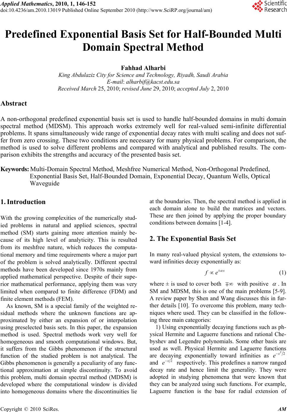Applied Mathematics, 2010, 1, 146-152
doi:10.4236/am.2010.13019 Published Online September 2010 (http://www.SciRP.org/journal/am)
Predefined Exponential Basis Set for Half-Bounded Multi
Domain Spectral Method
Fahhad Alharbi
King Abdulaziz City for Science and Technology, Riyadh, Saudi Arabia
Received March 25, 2010; revised June 29, 2010; accepted July 2, 2010
Abstract
A non-orthogonal predefined exponential basis set is used to handle half-bounded domains in multi domain
spectral method (MDSM). This approach works extremely well for real-valued semi-infinite differential
problems. It spans simultaneously wide range of exponential decay rates with multi scaling and does not suf-
fer from zero crossing. These two conditions are necessary for many physical problems. For comparison, the
method is used to solve different problems and compared with analytical and published results. The com-
parison exhibits the strengths and accuracy of the presented basis set.
Keywords: Multi-Domain Spectral Method, Meshfree Numerical Method, Non-Orthogonal Predefined,
Exponential Basis Set, Half-Bounded Domain, Exponential Decay, Quantum Wells, Optical
Waveguide
1. Introduction
With the growing complexities of the numerically stud-
ied problems in natural and applied sciences, spectral
method (SM) starts gaining more attention mainly be-
cause of its high level of analyticity. This is resulted
from its meshfree nature, which reduces the computa-
tional memory and time requirements where a major part
of the problem is solved analytically. Different spectral
methods have been developed since 1970s mainly from
applied mathematical perspective. Despite of their supe-
rior mathematical performance, applying them was very
limited when compared to finite difference (FDM) and
finite element methods (FEM).
As known, SM is a special family of the weighted re-
sidual methods where the unknown functions are ap-
proximated by either an expansion of or interpolation
using preselected basis sets. In this paper, the expansion
method is used. Spectral methods work very well for
homogeneous and smooth computational windows. But,
it suffers from the Gibbs phenomenon if the structural
function of the studied problem is not analytical. The
Gibbs phenomenon is generally a peculiarity of any func-
tional approximation at simple discontinuity. To avoid
this problem, multi domain spectral method (MDSM) is
developed where the computational window is divided
into homogeneous domains where the discontinuities lie
at the boundaries. Then, the spectral method is applied in
each domain alone to build the matrices and vectors.
These are then joined by applying the proper boundary
conditions between domains [1-4].
2. The Exponential Basis Set
In many real-valued physical system, the extensions to-
ward infinities decay exponentially as:
x
f
e


 (1)
where ± is used to cover both  with positive

. In
SM and MDSM, this is one of the main problems [5-9].
A review paper by Shen and Wang discusses this in fur-
ther details [10]. To overcome this problem, many tech-
niques where used. They can be classified in the follow-
ing three main categories:
1) Using exponentially decaying functions such as ph-
ysical Hermite and Laguerre functions and rational Che-
byshev and Legendre polynomials. Some other basis are
used as well. Physical Hermite and Laguerre functions
are decaying exponentially toward infinities as 22x
e
and 2
x
e respectively. This predefines a narrow ranged
decay rate and hence limit the generality. They were
adopted in studying phenomena that were known that
they can be analyzed using such functions. For example,
Laguerre function is the base for radial extension of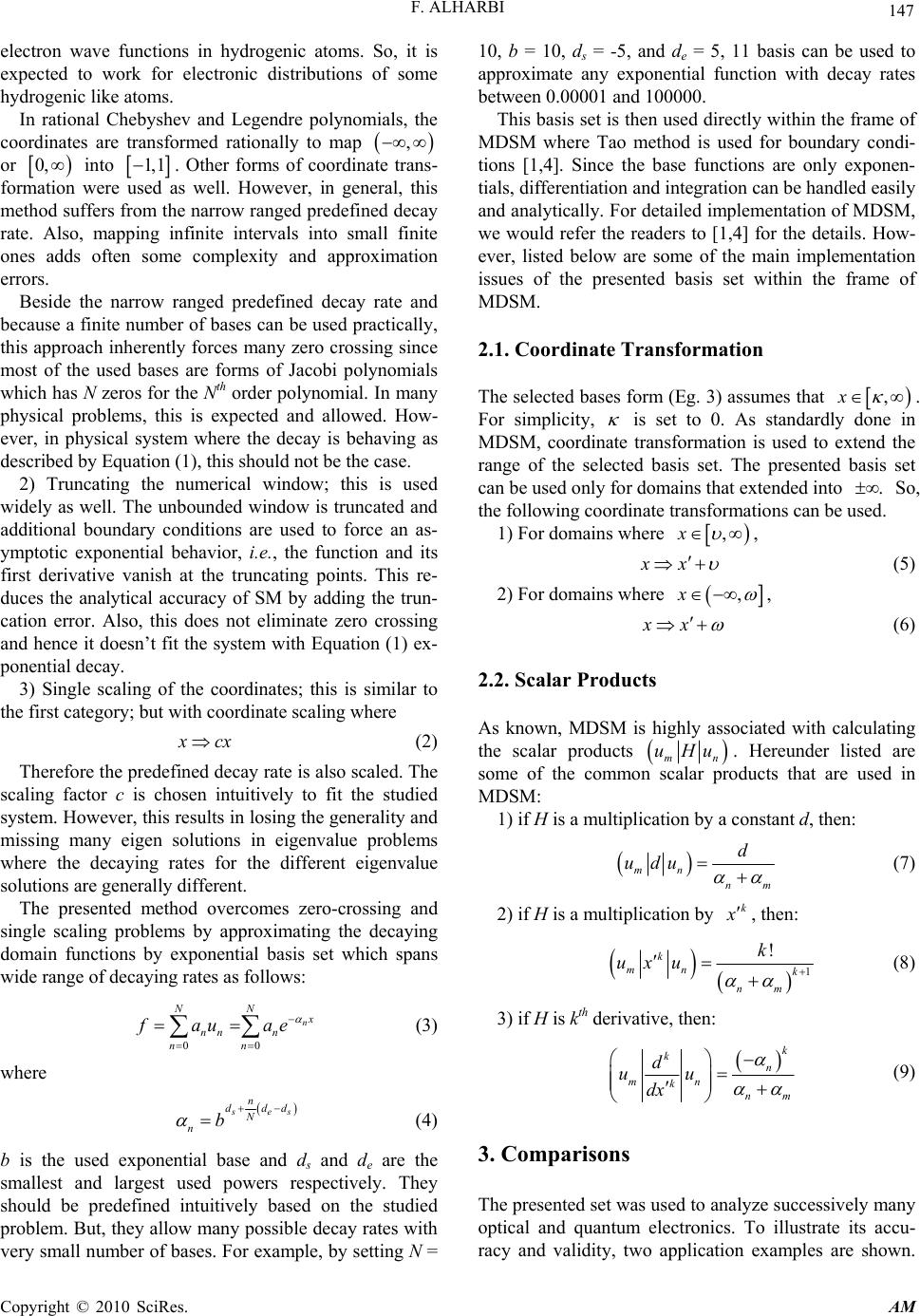

F. ALHARBI
147
electron wave functions in hydrogenic atoms. So, it is
expected to work for electronic distributions of some
hydrogenic like atoms.
In rational Chebyshev and Legendre polynomials, the
coordinates are transformed rationally to map


,


or


0, into


1,1. Other forms of coordinate trans-
formation were used as well. However, in general, this
method suffers from the narrow ranged predefined decay
rate. Also, mapping infinite intervals into small finite
ones adds often some complexity and approximation
errors.
Beside the narrow ranged predefined decay rate and
because a finite number of bases can be used practically,
this approach inherently forces many zero crossing since
most of the used bases are forms of Jacobi polynomials
which has N zeros for the Nth order polynomial. In many
physical problems, this is expected and allowed. How-
ever, in physical system where the decay is behaving as
described by Equation (1), this should not be the case.
2) Truncating the numerical window; this is used
widely as well. The unbounded window is truncated and
additional boundary conditions are used to force an as-
ymptotic exponential behavior, i.e., the function and its
first derivative vanish at the truncating points. This re-
duces the analytical accuracy of SM by adding the trun-
cation error. Also, this does not eliminate zero crossing
and hence it doesn’t fit the system with Equation (1) ex-
ponential decay.
3) Single scaling of the coordinates; this is similar to
the first category; but with coordinate scaling where
x
cx (2)
Therefore the predefined decay rate is also scaled. The
scaling factor c is chosen intuitively to fit the studied
system. However, this results in losing the generality and
missing many eigen solutions in eigenvalue problems
where the decaying rates for the different eigenvalue
solutions are generally different.
The presented method overcomes zero-crossing and
single scaling problems by approximating the decaying
domain functions by exponential basis set which spans
wide range of decaying rates as follows:
00
n
NN
x
nn n
nn
fauae
 


 (3)
where

s
es
n
ddd
N
nb


 (4)
b is the used exponential base and ds and de are the
smallest and largest used powers respectively. They
should be predefined intuitively based on the studied
problem. But, they allow many possible decay rates with
very small number of bases. For example, by setting N =
10, b = 10, ds = -5, and de = 5, 11 basis can be used to
approximate any exponential function with decay rates
between 0.00001 and 100000.
This basis set is then used directly within the frame of
MDSM where Tao method is used for boundary condi-
tions [1,4]. Since the base functions are only exponen-
tials, differentiation and integration can be handled easily
and analytically. For detailed implementation of MDSM,
we would refer the readers to [1,4] for the details. How-
ever, listed below are some of the main implementation
issues of the presented basis set within the frame of
MDSM.
2.1. Coordinate Transformation
The selected bases form (Eg. 3) assumes that


,x 

.
For simplicity,

is set to 0. As standardly done in
MDSM, coordinate transformation is used to extend the
range of the selected basis set. The presented basis set
can be used only for domains that extended into .

 So,
the following coordinate transformations can be used.
1) For domains where


,x 

,
xx



(5)
2) For domains where


,x

 ,
xx


 (6)
2.2. Scalar Products
As known, MDSM is highly associated with calculating
the scalar products


mn
uHu . Hereunder listed are
some of the common scalar products that are used in
MDSM:
1) if H is a multiplication by a constant d, then:

mn
nm
d
udu


 (7)
2) if H is a multiplication by k
x
, then:


1
!
k
mn k
nm
k
uxu


 (8)
3) if H is kth derivative, then:

k
k
n
mn
k
nm
d
uu
dx



 





(9)
3. Comparisons
The presented set was used to analyze successively many
optical and quantum electronics. To illustrate its accu-
racy and validity, two application examples are shown.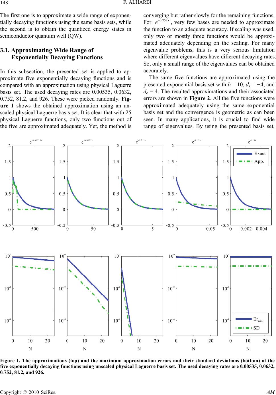

F. ALHARBI
148
The first one is to approximate a wide range of exponen-
tially decaying functions using the same basis sets, while
the second is to obtain the quantized energy states in
semiconductor quantum well (QW).
3.1. Approximating Wide Range of
Exponentially Decaying Functions
In this subsection, the presented set is applied to ap-
proximate five exponentially decaying functions and is
compared with an approximation using physical Laguerre
basis set. The used decaying rates are 0.00535, 0.0632,
0.752, 81.2, and 926. These were picked randomly. Fig-
ure 1 shows the obtained approximation using an un-
scaled physical Laguerre basis set. It is clear that with 25
physical Laguerre functions, only two functions out of
the five are approximated adequately. Yet, the method is
converging but rather slowly for the remaining functions.
For 0.752
x
e, very few bases are needed to approximate
the function to an adequate accuracy. If scaling was used,
only two or mostly three functions would be approxi-
mated adequately depending on the scaling. For many
eigenvalue problems, this is a very serious limitation
where different eigenvalues have difierent decaying rates.
So, only a small range of the eigenvalues can be obtained
accurately.
The same five functions are approximated using the
presented exponential basis set with b = 10, ds = −4, and
de = 4. The resulted approximations and their associated
errors are shown in Figure 2. All the five functions were
approximated adequately using the same exponential
basis set and the convergence is geometric as can been
seen. In many applications, it is crucial to find wide
range of eigenvalues. By using the presented basis set,
Figure 1. The approximations (top) and the maximum approximation errors and their standard deviations (bottom) of the
five exponentially decaying functions using unscaled physical Laguerre basis set. The used decaying rates are 0.00535, 0.0632,
0.752, 81.2, and 926.

F. ALHARBI
149
Figure 2. The approximations (top) and the maximum approximation errors and their standard deviations (bottom) of the
five exponentially decaying functions using the presented basis set with the same bases. The used decaying rates are 0.00535,
0.0632, 0.752, 81.2, and 926.
this can be done explicitly.
The presented set is used also to approximate wider
spectrum of decaying rates using the same bases. The
used decaying rates in this analysis are 1:35 × 10-6, 2.32
× 10-4, and 3:2, and 4120, and 526000. Again, these were
picked randomly. In this analysis, the used parameters
are b = 10, ds = −6, and de = 6. Figure 3 shows the ob-
tained approximations and their associated errors. It is
clear that the approximation is very efficient for all the
functions even with this wider spectrum of decaying
rates.
3.2. Single Semiconductor QW without
Biasing Field
In this subsection, a semiconductor quantum well is ana-
lyzed by MDSM and using the presented basis set. Elec-
tronic states in QWs are described by the envelopes of
the Bloch wave function. These are the solutions of the
effective mass approximation of Schrodinger wave equa-
tion, which is:

 
21
2
dx
dVx xx
dx dx mx







 (10)
where  is the normalized Planck constant,


mx

is
the effective mass, V(x) is the QW potential in the
growth direction, which is assumed to be the x-axis, 
is the quantized energy level, and

x

is the quantized
state. The studied structure is simply a thin layer of GaAs
sandwiched in Al0.3Ga0.7As. The width of the QW layer
is 20 nm. The structure is divided into three domains and
the structural parameters and the selected expansion ba-
sis sets in each domain are shown in the Table 1. This
structure can be analyzed analytically, where the energy
states are the solutions of the following characteristic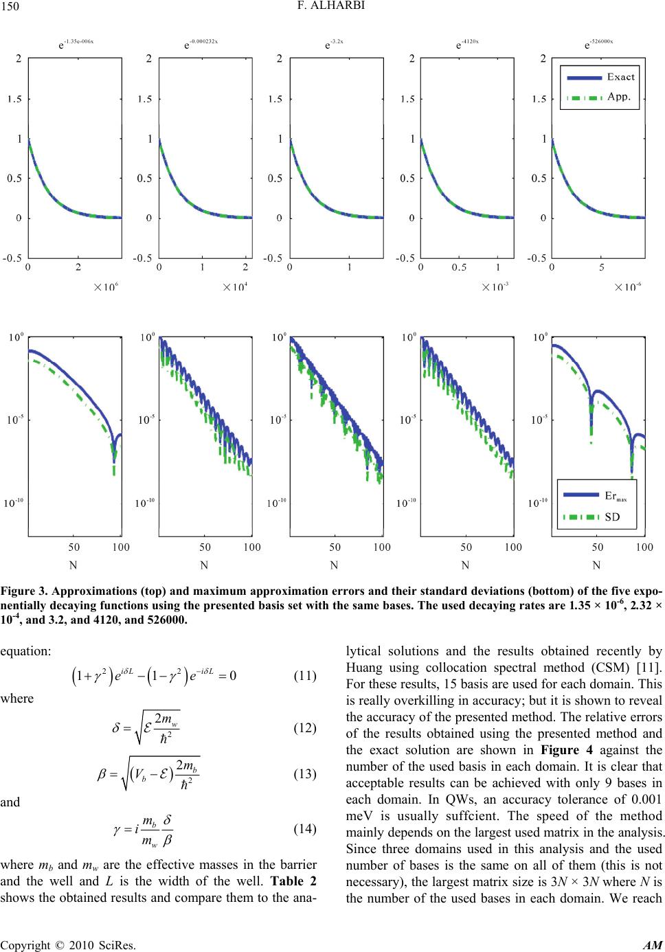

F. ALHARBI
150
Figure 3. Approximations (top) and maximum approximation errors and their standard deviations (bottom) of the five expo-
nentially decaying functions using the presented basis set with the same bases. The used decaying rates are 1.35 × 10-6, 2.32 ×
10-4, and 3.2, and 4120, and 526000.
equation:

22
11 0
iL iL
ee



 
(11)
where
2
2w m
   (12)

2
2b
b
m
V
 

 (13)
and
b
w
m
im



 (14)
where mb and mw are the effective masses in the barrier
and the well and L is the width of the well. Table 2
shows the obtained results and compare them to the ana-
lytical solutions and the results obtained recently by
Huang using collocation spectral method (CSM) [11].
For these results, 15 basis are used for each domain. This
is really overkilling in accuracy; but it is shown to reveal
the accuracy of the presented method. The relative errors
of the results obtained using the presented method and
the exact solution are shown in Figure 4 against the
number of the used basis in each domain. It is clear that
acceptable results can be achieved with only 9 bases in
each domain. In QWs, an accuracy tolerance of 0.001
meV is usually suffcient. The speed of the method
mainly depends on the largest used matrix in the analysis.
Since three domains used in this analysis and the used
number of bases is the same on all of them (this is not
necessary), the largest matrix size is 3N × 3N where N is
the number of the used bases in each domain. We reach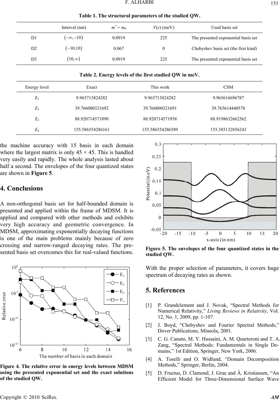

F. ALHARBI
151
Table 1. The structural parameters of the studied QW.
Interval (nm) m* = m0 V(x) (meV) Used basis set
D1

,10  0.0919 225 The presented exponential basis set
D2

10,10 0.067 0 Chebyshev basis set (the first kind)
D3

10, 0.0919 225 The presented exponential basis set
Table 2. Energy levels of the first studied QW in meV.
Energy level Exact This work CSM
E1 9.965713824282 9.965713824282 9.965616696787
E2 39.766000321692 39.766000321691 39.765614440578
E3 88.920714571890 88.920714571958 88.9198632662562
E4 155.586554286161 155.586554286589 155.585132856243
the machine accuracy with 15 basis in each domain
where the largest matrix is only 45 × 45. This is handled
very easily and rapidly. The whole analysis lasted about
half a second. The envelopes of the four quantized states
are shown in Figure 5.
4. Conclusions
A non-orthogonal basis set for half-bounded domain is
presented and applied within the frame of MDSM. It is
applied and compared with other methods and exhibits
very high accuracy and geometric convergence. In
MDSM, approximating exponentially decaying functions
is one of the main problems mainly because of zero
crossing and narrow-ranged decaying rates. The pre-
sented basis set overcomes this for real-valued functions.
Figure 4. The relative error in energy levels between MDSM
using the presented exponential set and the exact solutions
of the studied QW.
Figure 5. The envelopes of the four quantized states in the
studied QW.
With the proper selection of parameters, it covers huge
spectrum of decaying rates as shown.
5. References
[1] P. Grandclement and J. Novak, “Spectral Methods for
Numerical Relativity,” Living Reviews in Relativity, Vol.
12, No. 1, 2009, pp. 1-107.
[2] J. Boyd, “Chebyshev and Fourier Spectral Methods,”
Dover Publications, Mineola, 2001.
[3] C. G. Canuto, M. Y. Hussaini, A. M. Quarteroni and T. A.
Zang, “Spectral Methods: Fundamentals in Single Do-
mains,” 1st Edition, Springer, New York, 2006.
[4] A. Toselli and O. Widlund, “Domain Decomposition
Methods,” Springer, Berlin, 2004.
[5] D. Fructus, D. Clamond, J. Grue and Â. Kristiansen, “An
Efficient Model for Three-Dimensional Surface Wave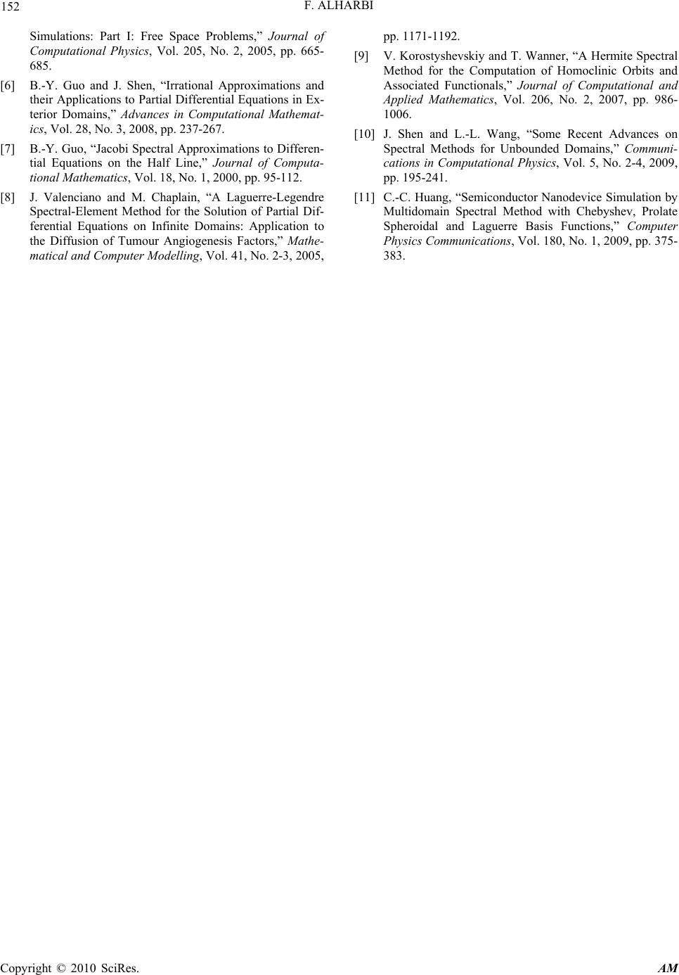

F. ALHARBI
152
Simulations: Part I: Free Space Problems,” Journal of
Computational Physics, Vol. 205, No. 2, 2005, pp. 665-
685.
[6] B.-Y. Guo and J. Shen, “Irrational Approximations and
their Applications to Partial Differential Equations in Ex-
terior Domains,” Advances in Computational Mathemat-
ics, Vol. 28, No. 3, 2008, pp. 237-267.
[7] B.-Y. Guo, “Jacobi Spectral Approximations to Differen-
tial Equations on the Half Line,” Journal of Computa-
tional Mathematics, Vol. 18, No. 1, 2000, pp. 95-112.
[8] J. Valenciano and M. Chaplain, “A Laguerre-Legendre
Spectral-Element Method for the Solution of Partial Dif-
ferential Equations on Infinite Domains: Application to
the Diffusion of Tumour Angiogenesis Factors,” Mathe-
matical and Computer Modelling, Vol. 41, No. 2-3, 2005,
pp. 1171-1192.
[9] V. Korostyshevskiy and T. Wanner, “A Hermite Spectral
Method for the Computation of Homoclinic Orbits and
Associated Functionals,” Journal of Computational and
Applied Mathematics, Vol. 206, No. 2, 2007, pp. 986-
1006.
[10] J. Shen and L.-L. Wang, “Some Recent Advances on
Spectral Methods for Unbounded Domains,” Communi-
cations in Computational Physics, Vol. 5, No. 2-4, 2009,
pp. 195-241.
[11] C.-C. Huang, “Semiconductor Nanodevice Simulation by
Multidomain Spectral Method with Chebyshev, Prolate
Spheroidal and Laguerre Basis Functions,” Computer
Physics Communications, Vol. 180, No. 1, 2009, pp. 375-
383.