International Journal of Modern Nonlinear Theory and Application, 2012, 1, 125-129
http://dx.doi.org/10.4236/ijmnta.2012.14019 Published Online December 2012 (http://www.SciRP.org/journal/ijmnta)
Stability Behavior of the Zero Solution for Nonlinear
Damped Vectorial Second Order Differential Equation
Mohamed A. Ramadan1, Samah M. El-Kholy2
1Department of Mathematics, Faculty of Science, Minufiya University, Shebeen El-koom, Egypt
2Department of Engineering Physics and Mathematics, Faculty of Engineering, Kafr El-Sheikh University, Kafr El-Sheikh, Egypt
Received October 7, 2012; revised November 9, 2012; accepted November 18, 2012
ABSTRACT
In this paper, a theoretical treatment of the stability behavior of the zero solution of nonlinear damped oscillator in the
vectorial case is investigated. We study the sufficient conditions for the boundedness of solution of the nonlinear
damped vectorial oscillator and the conditions for the stability of the zero solution to be uniformly stable as well as as-
ymptotically stable.
Keywords: Zero Solution; Damped Oscillator; Uniformly Stable; Asymptotically Stable
1. Introduction
We consider the nonlinear second order vectorial differ-
ential equation of the form
 
2,ftt t 
  xxxgx0
.R
(1)
where;

 
12
,,,
,:,and, :
,,
n
n
nn
tRxxx R
tRRR fttR 


 
 
x
gx
Stability problems for the second order ordinary differ-
ential equation has been intensively and widely studied
[1-5]. Based on Schauder fixed point theorem T. A. Bur-
ton and T. Furumochi [2] introduced a new method to
study the stability of the zero solution for Equation (1).
This problem is considered also by Gheorghe Morosanu
and Cristian Vladimirescu [5,6]. In [6], they used rela-
tively classical arguments to prove the stability of the
zero solution of Equation (1). While in [5], they obtained
new stability results for this ordinary differential equa-
tion under more general assumptions. Their approach al-
lows extensions to both the vector case and the case of
the whole real line. In [7] the dynamics of various oscil-
lators had been studied.
2. The Main Results
In the next theorem we state sufficient conations for the
boundedness of the solution of Equation (1) are given.
Theorem 1
If the following hypotheses are hold:
1)


1
f
tCR

 and


0, 0ft t.
2)




1,tCR




is decreasing and


1t  ,
tR

 .
3)


n
R,
n
CR R

g and
g is locally Lipschit- zian
in


1,, n
x
x,
4) g satisfies the following estimate






,tfto
g
xx
, , where tR

  denotes
some norm in . then the solution of Equation (1) is
bounded.
n
R
Proof
For the n-dimensional system, we have

T
12 12
,,,,,,, m
nn
x
xxyyy Rz, where m = 2n.
Applying the transformation,


ii i
y
xftx

 and
1, 2,,in

 Equation (1) can be converted into a first
order system of differential equations of the form:




,

A
tBt t

zzzrz (2)
where
1)





 
12
34
A
tAt
At
A
tAt






 and are
m × m matrices.
 
1
00
0
Bt Bt



2)






14
A
tAt ftI,

2
A
tI,




3
A
ttI   , and


2
f tf
 


t I
1
Bt
0nn
are n ×
n matrices. Note that,

and I are the zero and the
identity matrices, respectively.
3)
 
T
1
,0 ,,
n
tgtgt

 


rxx x

1
0
,
n
t







gx
which is a 2m1

vector.
For ,1,2,,ij n

, let is an arbitrary fixed
and let
00t
C
opyright © 2012 SciRes. IJMNTA

M. A. RAMADAN, S. M. EL-KHOLY
126






 
 
11 012010
,,
21 022020
0
,,
10 0
,, ,
,, ,
,
,,
m
ijin j
m
nijnin j
mm m
zttzttz tt
ZZ
zttzttztt
Ztt ZZ
zttz tt






















(3)
be a fundamental matrix solution to the linear system:


A
t
zz (4)
which equal to the identity matrix for .
0
Consider with
tt
00z0
z small enough, and
let us denote by
00t


00
,,ttzz
0
z the unique solution of Equa- tion (2) which equal to

at . By hypotheses (1)
0
tt
and (2),


0
z
0
,,ttz is defined on a maximal right inter-
val,


0,tl, and satisfies the following integral equation:
     
0
1
000 0000000
,,,,,,,, ,,d
t
t
ttZ ttZ ttZstBsstssts



 



zzzzzrzz
This gives us the following integral inequality:
    
0
1
000 0000000
,,,,,e,,,,,d
t
t
ttZ ttZ ttZstBsstssts



 



zzzzzrzz (5)
where .

T
010e
Equations (3) and (4) give us the following differential
equations:

,,ijij nij
zftzz

 ,
,
,
,
(6)
 
,,nijij nij
ztzftz 

  (7)

,,injinj ninj
zftzz

 (8)
 
,,nin jin jninj
ztzftz 
 
  (9)
for . ,1,2,,ij n


Since is a decreasing function, so Equations (6)
and (7) lead to:
t
 
22 22
,, ,,
1
2ij nijij nij
tz zfttzz 



 




0
2d
22
,, 0
e
t
t
f
uu
ij nij
tz zt 



 (10)
By the same way we can obtain from Equations (8)
and (9) the following:


0
2d
22
,,
e
t
t
f
uu
in jnin j
tz z 



 (11)
For

T
12 12
,,,,,,, m
nn
x
xxyyy Rz, consider
the norm 2
1
m
i
i
z



z, where  is the norm defined
in .
m
R


For

T
001 02001020
,,,,,,, m
nn
x
xxyyy Rz we
have:

 
,, ,0,0 0
00
,, ,0,0 0
22
,0,0,0, 0
11 1
,ijin jijin j
nijnin jnijnin j
nn n
ijjinjjnijjnin jj
ij j
ZZZZ
Ztt ZZZ Z
zx zyzx zy

 

 

 


 










 
xy
x
zxy
y



satisfies (4), then we get: Using Shwartz inequality, Minkowski inequality [8] and
suitable assumptions lead to:
 

0
2d
00 00
,31e
t
tfu u
Zttn t 


z
z (12)
We have also:
00tst 

 
1
00
T
1020 0
,,e
,, ,,,,
m
Ztt Zst
tst tsttst  

  


  

1
00
0
1
22
00
1
,,e
,, ,,
i
i
n
ii n
i
Ztt Zst
ttsttst
 






Since
2,,
mtst
 


t  is a decreasing function of , we get:
t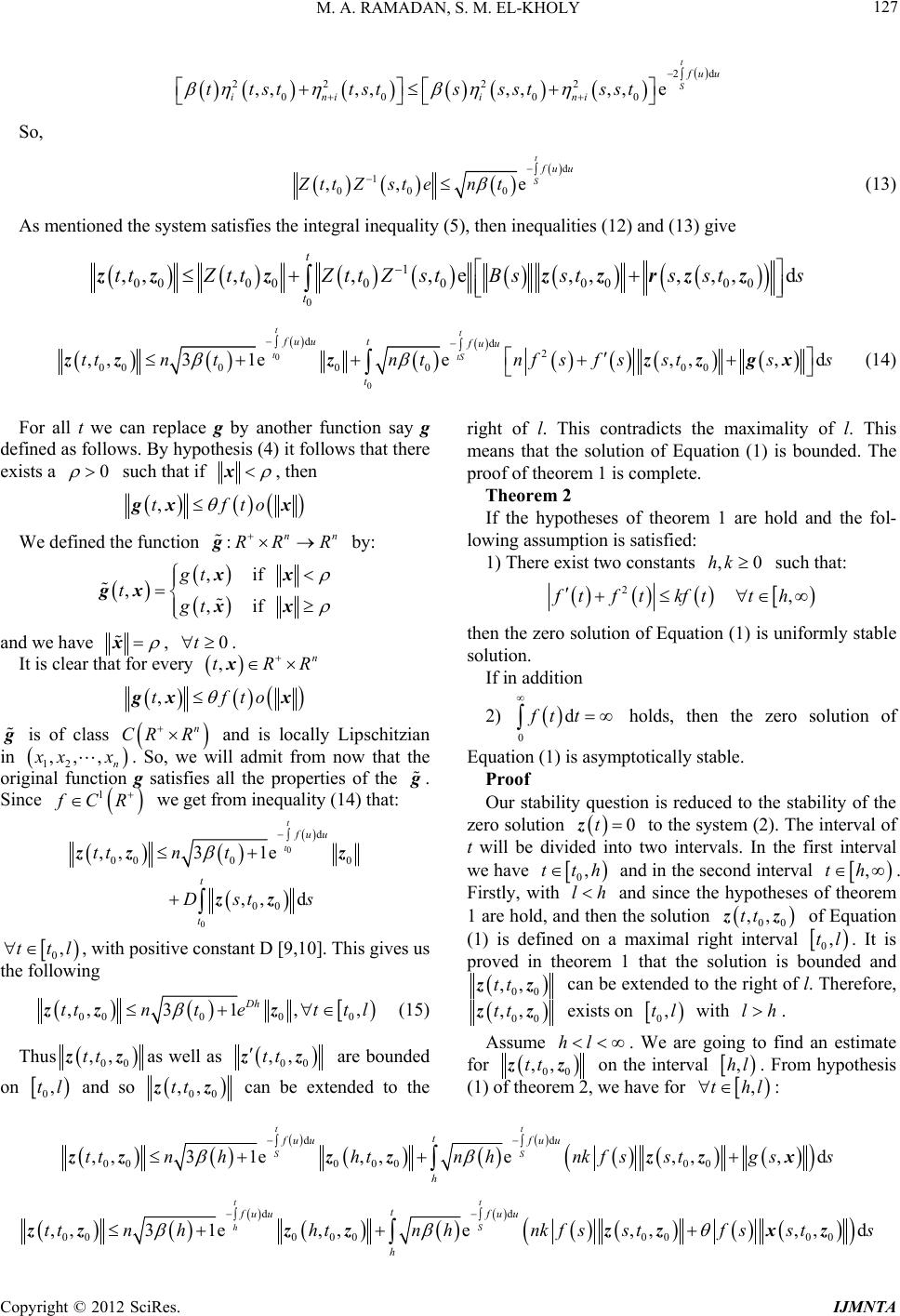

M. A. RAMADAN, S. M. EL-KHOLY 127



 
22 2 2
0000
,,,,,,,,e S
 2d
t
f
uu
in
i ini
t tsttsts sstsst  


 



So,
  

d
1
00 0
,, e
t
S
fu u
Ztt Zstent 


 (13)
As mentioned the system satisfies the integral inequality (5), then inequalities (12) and (13) give
 

 

0
1
0000000000
,,,,,e,,,,,d
t
t
ttZ ttZ ttZstBsstssts







 

zzzzzrzz
 






0
dd
2
0000 000
,,31ee
tt
ttS
fu utfuu
ttntn tnfs 


0
t
,,,df sstss


  



zz z
For all t we can replace g by another function say g
defined as follows. By hypothesis (4) it follows that there
exists a
zzgx (14)
0

 such that if

x, then




,tfto  gx x
We defined the function by:
:nn RRR


g
 

,if
,,if
gt
tgt



ave






xx
gx xx
and we h



x, t0.
ry ,x It is clear that for eveR

tR


n




,tgx fto  x
is of class and is locally Lipschitzian
 g
in

n
CR R


n12
,,,
x
xx
ginal function
. So, we w
g satisfies

ill admit from now that the
all the properties of the ori  g.
Since 1
f
CR
 we get from inequality (14) that:
 


0
00 0 0
,,31e
t
tfu
t
ttn t
D




0
00
,, d
t
s
t s
du
z
zz
u
g
zz


0,ttl , with positive constant D [9,10]. This givess
the followin
   
0000 0
,,31 ,,
Dh
ttntett l  zzz (15)
Thus

00
,,tt
z
zas well as

00
,,tt

z
z are bounded
on and so
 
0,tl

00
,,tt
z
z can be extended to the
right of l. This contradicts the maximality of l. This
means that the solution of Equation (1) is bonded. The
proof of theorem 1 is complete.
Theorem 2
If the hypotheses of theorem 1 are hold and
lowing assumption is satisfied:
1) There exist two constants such that:
u
the fol-
,0hk






2,ftf tkftth



then the zero solution of Equation (1) is uniformly stable
solution.
If in addition

2)

0
dft t


 holds, thzero solution en the of
Equation (1) is asymptotically stable.
Proof
n
Our stability question is reduced to the stability of the
zero solutio


0t

z
will be divided into two intervals. In the
to the system (2). The interval of
tfirst interval
we have


0,tth and in the second interval


,th

.
lh

and si
on a ma
Firstly, with nce the hypotheses of theorem
1 are hold, and then the solution

,tz

of Equation
00
,tz
l right interval (1xima) is defined


0,tl. It is
proved in theorem 1 that the solution is bounded and


00
,,tt
z
z cantended to the right of l. Therefore, be ex


00
,,tt
z
z exists on


0,tl with lh.
Assume hl

. We are going to find an estimate
for


00
,,tt
z
z on the interval
 
,hl . From hypothesis
(1) of theorem 2, we have for thl :

,

 

 

  

,,, d
t
unk fsstgsszz x dd
000 0
,,31e,e
t
SS
t
fuufu
ttnhhtnh 


 zzz z
0
,
h
00
 

 

   

dd
0
, ,
t
hS
fu u
nhnkfs fs

z z
00 00
h
00 00
e,,,, d
t
fu ustst s


zzxz ,3 1e,
t
tthtn h 



z z

M. A. RAMADAN, S. M. EL-KHOLY
128
with

1
0, nk
nh






(16)






  

00
d
000
d
00
,,
31e ,,
e
t
h
t
S
fuu
tfuu
h
tt
nh ht
nhnkfs sts









zz
zz
zz , ,d
(17)
 




  
d
000
d
00
31e ,,
e,
t
h
t
S
fuu
tfuu
h
vt hht
nhnkfssts









zz
zz
So
,d
 


1,vtnh nkftvtthl 


 .
By integration we get:
  
 
 
1d
00
,,e ,
,
t
h
nhnk fuu
ttt h
thl
vv






zz (18
with
)
 

00
31,,vh nhht  zz
From inequality (18) we can see that

00
,,tt
z
z is
bounded since

00
,,tt

z
z is also bounded, it folls
that For
ow
l .0

 we can get:
 



2
e
13013
Dh
nh






From (15) it follows that


00
,,
13
tt nh


 zz
for all


0,tth provided that 0

zore,
from (16) and (1t

. Theref
, we ge8)

00
,,ttvh

zz for
all th o, if h, then the solution . S00 t


starting
00
,,ttzz
from any point 0
z
, with 0

z, exists on

0
t

, and satisfies

00
,,tt

zz for al
usly we btain that
l 0 tt. If
and:
0
th, then analogool
 
 

0
1d
0
e ,
t
nhnkfuu 





(19

,th
Therefore, with the same
00 0
,,31ttnt  zz z)
t

as before, 0


z im-
plies again

00
,,tt

zHence the
If in
z for all 0 tt.
zero solution is uniformly stable.
addition


0
dft t



is satisfied, then by (16), (18) and (19) it follows tha
zero solution to (1) is asymptotically stable. The proof of
theorem 2 is complete.
3. Examples
We confirm the results of the introduced theorems by
considering two numerical examples for which the func-
tions
t the


f
t,


t  and


tg satisfy theorems assump-
tions.
For the system

 
2,ft t 
 

t0

 xxxgx
where
,


12
,
x
xx

.
Example 1

21
t
ft t 

,


11tt 

,

12
112 2
,, 1
x
xt
gtxxt 

and



22
12
212 2
,, 1
x
xt
gtxx t

.
(a)
(b)
Figure 1. Numerical solutions if Example 1, x1 component (a)
and x2 component (b).

M. A. RAMADAN, S. M. EL-KHOLY 129
(a)
(b)
Figure 2. Numerical solutions if example 2, x1 component (a)
and x2 component (b).
Example 2

2
1
ft t , ,

2
1e
t
t 



12
112 2
,,
x
x
gtxx t  and


22
12
2
212
,,
x
x
t

. gt xx
We solved these two examples numerically using
th order Runge-Kutta method. The results of example 1
are drawn as shown in Figure 1 and the results of exam-
own in Figure 2. The curves are
rawn for different initial values of
d 2 demonstrate time increases
all the compents of the solutions tends to zero.
means, that te aptotically stable. W
verify the rightness of our proved theorems.
4. Conclusion
ifo ly stable as well
as
REFERENCES
nd T. Furumochi, “A Note on Stability by
87.
[4] J. Hale, “Ordina,” Wiley Inter-
science, John Woken, 1969.
four-
ple 2 are drawn as sh
d0
x.
that, as the Figures 1 an
on This
he solutions arsymhich
We introduced two theorems which provide the sufficient
conditions for the boundedness of solution of the nonlin-
ear damped vectorial oscillator and the conditions for the
stability of the zero solution to be unrm
asymptotically stable. We verified our theoretical re-
sults by solving two examples satisfying the assumptions
of the two proved theorems.
[1] T. A. Burton a
Schauder’s Theorem,” Funkcialaj Ekvacioj, Vol. 44, No.
1, 2001, pp. 73-82.
[2] V. A. Coppel, “Stability and Asymptotic Behavior of Dif-
ferential Equations,” D. C. Heath and Company, Lexing-
ton, 1965.
[3] D. Grossman, “Introduction to Differential Equations with
Boundary Value Problems,” Wiley-Interscience, John Wiley
& Sons, Inc., Hoboken, 19
ry Differential Equations
iley & Sons, Inc., Hob
[5] G. H. Moroşanu and C. Vladimirescu, “Stability for a Non-
linear Second Order ODE,” Funkcialaj Ekvacioj, Vol. 48,
No. 1, 2005, pp. 49-56. doi:10.1619/fesi.48.49
[6] G. H. Moroşanu and C. Vladimirescu, “Stability for a
Damped Nonlinear Oscillator,” Nonlinear Analysis, Vol.
60, No. 2, 2005, pp. 303-310.
[7] J. Awrejcewicz, “Classical Mechanics. Dynamics,” Sprin-
ger-Verlag, New York, 2012,
[8] R. F. Curtain and A. J. Pritchard, “Functional Analysis in
l and Inte-
Modern Applied Mathematics,” Academic Press Inc. Ltd.,
London, 1977.
[9] R. Bellman, “Stability Theory of Differential Equations,”
Dover Publications Inc., Mineola, 1953.
[10] V. Lakshmikantham and S. Leela, “Differentia
gral Inequalities. Theory and Applications,” Academic
Press, New York and London, 1969.