J. Serv. Sci. & Management, 2009, 2: 43-46
Published Online March 2009 in SciRes (www.SciRP.org/journal/jssm)
43
Study on Measuring Methods of Real Estate Speculative
Bubble
Yifei Lai
1
, Huawei Xu
1
, Junping Jia
1
1
School of Economics and Management, WuhanUniversity, Wuhan, Hubei, China.
Received December 18
th
, 2008; revised January 14
th
, 2009; accepted February 5
th
, 2009.
ABSTRACT
The paper analyses the causes of the bubble of the real estate, then elaborates real estate bubble theory based on specu-
lation. This paper establishes a regression model of real estate’s price with relevant economic variables, and builds the
econometric model to measure real estate’s speculative bubble. In application of the model for empirical research on
real estate’s speculative bubble of Chongqing, the paper concludes that globally there is no bubble in Chongqing (but
on the edge of bubble). Finally, by analyzing the common points about the existence of bubble, the paper indicates that
real estate’s investment and macro-economic indexes are disjointed, and thus the investment is excessive, which can in
turn corroborate the conclusions obtained by the measuring model.
Keywords: real estate, speculative bubble, measuring model of speculative bubble, overinvestment
1. Introduction
At present, China is under the pressure of high inflation,
and real estate price soared quickly. From 2005 to 2007,
the government adopted a series of macro-control poli-
cies, for example, in March 2005, “country’s 8 items”
came out, so that the regulation of real estate was boosted
to a high degree of polity; in April 2006, mortgage inter-
est rate rose again; in May, “country’s 6 items” came out,
then waged a new round of large-scale control; at the
same period, China begun to impose tax on second-hand
estate’s sales; in July, China begun to impose personal
income tax of transferring second-hand estate; in Sep-
tember, down payment rose. However, the real estate
industry continues to show strong-run tendency, real es-
tate price remains high. The real estate industry is highly
relevant to many other industries, and its positive run can
promote the development of other industries. Otherwise,
if the real estate industry goes against the Law of value of
market, its price separates from the market base but keeps
irrational growth, the bubble is inevitable, and when the
bubble has expanded to a certain degree to leak, then the
financial system will bear the brunt, and even the national
economy will experience turbulence. In 1997, the break-
down of real estate speculative bubble plunged Japan into
stagnant economic downturn. Thus, it is of great signifi-
cance to measure the speculative bubble of the current real
estate market and identify the over-investment. Chongqing’s
real estate was selected as an example to measure its specu-
lative bubble applying the proposed methods.
2. The Theory and Measuring Model
2.1 Real Estate Bubble Based on Speculative
Theory
According to the reasons of real estate bubble, under the
effect of consumer expectation, there are many positive
feedback effects, namely, investors dealing according to
the tendency of past asset price, not to the real price.
Thus, we can consider, positive feedback deal determines
the change of future demand in real estate market, and
then the expectation of future real estate price in market
is determined by the expectation of future change of de-
mand. Firstly, when the increasing rate of real estate price
exceeds credit loan rate, the real estate price speculation
comes out. At this time, investors achieve speculative
aim by changing hand to get the price difference; sec-
ondly, there is time interval between buying and selling,
which provides speculative possibility. At last, because of
the imperfection of market mechanism and information
asymmetries, the price arbitrage action of speculators will
result in the achievement of expectation.
2.2 The Measuring Model of Real Estate
Speculative Bubble
In terms of positive feedback mechanism, real estate price
at current period will be affected by past several real estate
price. Considering that speculations are general short-term
price arbitrage action by selling real estate, because specu-
lators are not aiming to achieve the steady long-term profit
in the future, e.g., earning rents after buying estate.
Let
t
h
figures real increasing rate of real estate price
at period t, which is achieved after eliminating the growth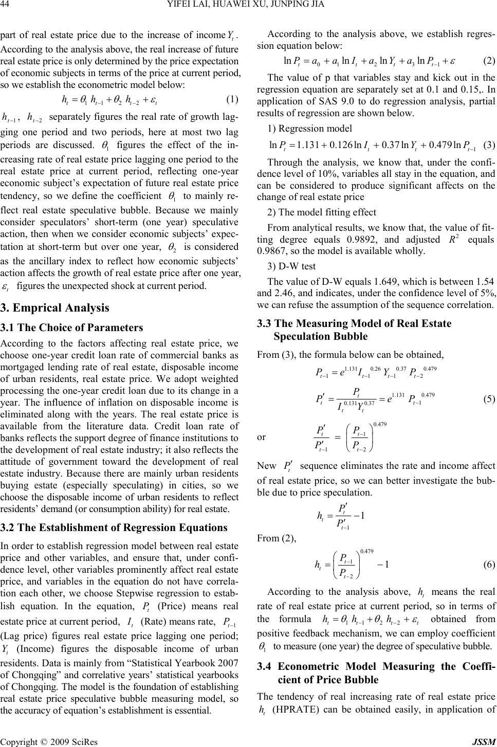

44 YIFEI LAI, HUAWEI XU, JUNPING JIA
part of real estate price due to the increase of income
t
Y
.
According to the analysis above, the real increase of future
real estate price is only determined by the price expectation
of economic subjects in terms of the price at current period,
so we establish the econometric model below:
1 122
ttt t
h hh
θ θε
− −
= ++
(1)
1
t
h
−
,
2
t
h
−
separately figures the real rate of growth lag-
ging one period and two periods, here at most two lag
periods are discussed.
1
θ
figures the effect of the in-
creasing rate of real estate price lagging one period to the
real estate price at current period, reflecting one-year
economic subject’s expectation of future real estate price
tendency, so we define the coefficient
1
θ
to mainly re-
flect real estate speculative bubble. Because we mainly
consider speculators’ short-term (one year) speculative
action, then when we consider economic subjects’ expec-
tation at short-term but over one year,
2
θ
is considered
as the ancillary index to reflect how economic subjects’
action affects the growth of real estate price after one year,
t
ε
figures the unexpected shock at current period.
3. Emprical Analysis
3.1 The Choice of Parameters
According to the factors affecting real estate price, we
choose one-year credit loan rate of commercial banks as
mortgaged lending rate of real estate, disposable income
of urban residents, real estate price. We adopt weighted
processing the one-year credit loan due to its change in a
year. The influence of inflation on disposable income is
eliminated along with the years. The real estate price is
available from the literature data. Credit loan rate of
banks reflects the support degree of finance institutions to
the development of real estate industry; it also reflects the
attitude of government toward the development of real
estate industry. Because there are mainly urban residents
buying estate (especially speculating) in cities, so we
choose the disposable income of urban residents to reflect
residents’ demand (or consumption ability) for real estate.
3.2 The Establishment of Regression Equations
In order to establish regression model between real estate
price and other variables, and ensure that, under confi-
dence level, other variables prominently affect real estate
price, and variables in the equation do not have correla-
tion each other, we choose Stepwise regression to estab-
lish equation. In the equation,
t
P
(Price) means real
estate price at current period,
t
I
(Rate) means rate,
1
t
P
−
(Lag price) figures real estate price lagging one period;
t
Y
(Income) figures the disposable income of urban
residents. Data is mainly from “Statistical Yearbook 2007
of Chongqing” and correlative years’ statistical yearbooks
of Chongqing. The model is the foundation of establishing
real estate price speculative bubble measuring model, so
the accuracy of equation’s establishment is essential.
According to the analysis above, we establish regres-
sion equation below:
0 1231
lnln ln ln
tt t t
P aaIaY aP
ε
−
= ++++
(2)
The value of p that variables stay and kick out in the
regression equation are separately set at 0.1 and 0.15,. In
application of SAS 9.0 to do regression analysis, partial
results of regression are shown below.
1) Regression model
1
ln1.131 0.126ln0.37ln0.479ln
tt tt
PI YP
−
= +++ (3)
Through the analysis, we know that, under the confi-
dence level of 10%, variables all stay in the equation, and
can be considered to produce significant affects on the
change of real estate price
2) The model fitting effect
From analytical results, we know that, the value of fit-
ting degree equals 0.9892, and adjusted
2
R
equals
0.9867, so the model is available wholly.
3) D-W test
The value of D-W equals 1.649, which is between 1.54
and 2.46, and indicates, under the confidence level of 5%,
we can refuse the assumption of the sequence correlation.
3.3 The Measuring Model of Real Estate
Speculation Bubble
From (3), the formula below can be obtained,
1.131 0.260.370.479
11 12 tt tt
Pe IYP
−−− −
=
1.131 0.479
1
0.131 0.37
t
t t
t t
P
Pe P
I Y
−
′= = (5)
or
0.479
1
1 2
t t
t t
P P
P P
−
− −
′ 
= 
′ 
New
t
P
′
sequence eliminates the rate and income affect
of real estate price, so we can better investigate the bub-
ble due to price speculation.
1
1
t
t
t
P
hP
−
′
= −
′
From (2),
0.479
1
2
1
t
t
t
P
hP
−
−
 
= −
 
 
(6)
According to the analysis above,
t
h
means the real
rate of real estate price at current period, so in terms of
the formula
1 122
ttt t
h hh
θ θε
− −
= ++
obtained from
positive feedback mechanism, we can employ coefficient
1
θ
to measure (one year) the degree of speculative bubble.
3.4 Econometric Model Measuring the Coeffi-
cient of Price Bubble
The tendency of real increasing rate of real estate price
t
h
(HPRATE) can be obtained easily, in application of

YIFEI LAI, HUAWEI XU, JUNPING JIA 45
Figure 1. Trend of real increasing rate of real estate
price
t
h
(HPRATE) and first difference (HPRATE1)
time series
Eviews5.0 to conduct time series analysis, co-integration
test with HPRATE, we find that it is not integrative under
the level, after first difference, this time series (HPRATE1)
become a unit root series, and the trend chat of the two
are shown as following.
From the trend chart of HPRATE1, we know that, real
increasing rate of real estate price took on large fluctua-
tion in 1995, and then it fell to normal level in 1996, this
illustrated that there existed affective factors producing
large shock to real estate price, we consider that there
exists structure change. In fact, the investment of real
estate in our country between1992 and 1993 was ex-
ceeded, then in 1994, the government carried out
macro-control of our economy, “City Real Estate Man-
agement Law” coming out, leading economy to practice
soft landing. Considering the lag effect of macroeconom-
ics policy, we set dummy variable PL to reflect the shock
of policy.
Establish the following model:
1 122
t ttt
h hhPL
θθβ ε
− −
=++ +
(7)
From the table above, we get the model below:
HPRATE1=0.007 - 0.12 * PL+[AR(1)=-0.63,
MA(1)=0.91, BACKCAST=1992] (8)
(0.78) (-3.49) (-3.21)
Table 1. Eviews analysis results
Variable Coefficient Std. Error t-Statistic Prob.
C 0.006593 0.008439 0.781300 0.4511
PL -0.116048 0.033162 -3.499400 0.0050
AR(1) -0.631575 0.196634 -3.211928 0.0083
MA(1) 0.910039 0.049313 18.45421 0.0000
R-squared 0.723529 Durbin-Watson stat 1.96375
Obviously, the original model is:
1 2
0.007 0.120.370.63
tt t
hPL hh
− −
= −++ (9)
3.5 Results Analysis
From the results, we know that coefficient of real estate
speculation
1
θ
equals 0.37 which is close to the interna-
tional alertness line 0.4, but it is not at bubble level; an-
cillary index
2
θ
equals 0.63, which also reflects the
expectation (over one year) of economic subject in cer-
tain extent images bubble degree. Coefficient of policy
shock variable PL
β
equals - 0.12, which reflects that
the macroeconomics policy in 1994 well restrained real
estate speculation. So we can have following conclusion:
The real estate industry in Chongqing is on the edge of
bubble, but does not take on bubble, the macroeconomics
policies in 1994 worked. This conclusion basically ac-
cords with the reality of Chongqing.
3.6 Further Analysis of the Model Conclusion
From the conclusion of the model, we know that our
Chongqing is on the edge of bubble, but not has bubble,
but why there generally exist “bubble intimidation the-
ory”, “bubble perdition theory”. We support the conclu-
sion of speculation measuring model analysis by analyz-
ing the relation between real estate investment and mac-
roeconomics variable. We choose real estate investment
(REINV) and GDP of Chongqing, and also analyze the
relation of real estate investment and disposable income
(INCOME) of urban residents.
1) Co-integration test. Through ADF test, we find the
real estate investment (REINV2), GDP (GDP2, urban
residents’ income (INCOME2) are all 2-order integration
variables. Co-integration test uses M3 model and AIC
principle to choose lag order. The lag order is 3 periods
in co-integration test of REINV2 and GDP2, the value of
AIC is 13.11743; the lag order is 3 periods in the co-in-
tegration of REINV2 and GDP2, the value of AIC is
15.84799. The results of Co-integration test are shown in
Table 2.
2) Granger causality test. Because the three variables
are all 2-order integration variables, we can directly use
VAR model to conduct Granger causality test. We try to
choose different orders to study the sensitivity of the test
results, and the results are shown in Table 4.
-.02
.00
.02
.04
.06
.08
.10
.12
.14
1990 1992 1994 1996 1998 2000 2002 2004 2006
HPRATE
-.12
-.08
-.04
.00
.04
.08
1990 1992 1994 1996 1998 2000 2002 2004 2006
HPRATE1

46 YIFEI LAI, HUAWEI XU, JUNPING JIA
Table 2. REINV2 and INCOME2 Johansen co-integration test results
Count of Co- integration Equations Eiqenvalue T-Statistic 5% Critical Value prob.**
None 0.376550 9.292334 15.49471 0.3390
At most one 0.136708 2.205029 3.841466 0.1376
Count of Co-integration Equations Eiqenvalue Most Eiqenvalue Statistic 5% Critical Value prob.**
none 0.376550 7.087305 14.26460 0.4789
At most one 0.136708 2.205029 3.841466 0.1376
Table 3. REINV2 and GDP2 Johansen co-integration test results
Count of Co-integration equations Eiqenvalue T-Statistic 5% Critical Value prob.**
None 0.395752 10.20828 15.49471 0.2651
At most one 0.162037 2.651715 3.841466 0.1034
Count of Co-integration equations Eiqenvalue Most Eiqenvalue Statistic 5% Critical Value prob.**
None 0.395752 7.556565 14.26460 0.4256
At most one 0.162037 2.651715 3.841466 0.1034
Table 4. Two groups of variables’ Granger causality test results
Probability
Variables
0
H
(Null Hypothesis) Lag=1
Lag=2 Lag=3 Lag=4 Lag=5
0.726 0.643 0.32 0.790 0.884
REINV2-GDP2 GDP2 does not Granger Cause INVEST2
INVEST2 does not Granger Cause GDP2 0.074 0.109 0.016 0.137 0.413
0.777 0.997 0.258 0.540 0.312
REINV2-INCOME2 INCOME2 does not Granger Cause INVEST2
INVEST2 does not Granger Cause INCOME2 0.0001
0.005 0.033 0.157 0.418
From Table 3 and Table 4, we can get that under the
confidence level of 0.1, real estate investment, GDP and
the income of urban residents do not have co-integration,
which shows that real estate investment has been out of
the track of macroeconomic development, and overin-
vestment appears.
Table 4 further shows that under the confidence level
of 0.1, real estate investment and GDP, income only have
one-way causality. Real estate investment can promote
the growth of GDP and strongly promote income growth
in the short term, which once again indicates the exis-
tence of speculation which is short-term.
4. Conclusions
This paper empirically analyzes real estate speculative
bubble of Chongqing after establishing bubble measuring
model. The results indicate that Chongqing’s real estate
has not reached the bubble level, but is close to critical
value. The paper also analyzes the opinions of bubble theory
in the society, and empirical analysis pointes out that there is
excessive investment of real estate, which separates from the
growth of GDP and residents’ income in Chongqing. The
conclusion accordingly supports the empirical analysis re-
sults of speculative bubble measuring model.
Empirical analysis concludes that real estate of
Chongqing is on the verge of bubble, which offers con-
sultation for policymaker to work out corresponding
measures.
In addition, through macroeconomics regulation, the
government should scale down the investment of real
estate to the normal level, coordinate with macroeco-
nomics indexes of the region, to avoid excessive invest-
ment then to further induce expansion of bubble.
REFERENCES
[1] P. Wang, “Market efficiency and rationality in property
investment,” Journal of Real Estate Finance and Econom-
ics, 21(2): pp.185-200, 2000.
[2] C. Lizieri and S. Satchell, “Interacion between property
and equity markets: An investigation of linkages in the
UK 1972-1992,” Journal of Real Estate Finance and Eco-
nomics, 1997(15): pp.11-25, 1997.
[3] J. Abraham and P. H. Hendershott, “Bubbles in metro-
politan housing markets,” Housing Res, 1995(6): pp.
191-207, 1995.
[4] P. Bacon, F. Mac Cabe, and A. Murphy, “An economics
assessment of recent house price developments,” [M]
Government of Ireland Publication, Dublin, 1998.
[5] J. Eatwell, M. Milgate, and P. Newman, “The new pal-
grave: A dictionary of economics,” London Mac. Millan,
Vol. 1, pp. 28.
[6] K. H. Kim and H. S. Seoung, “Speculation and price bub-
bles in the korean and japanese real estate markets,”
Journal of Real Estate Finance and Economics [J],
1993(6): pp. 73-86.
[7] K. H. Kim and H. S. Lee, “Real estate price bubble and
price forecasts in Korea,” Proceedings of 5th AsRES
conference in Beijing, 2000.
[8] J. K. Zhou, “Financially support excessively and the real
estate bubble,” Beijing University Press, 2005.
[9] H. Y. Liu and H. Zhang, “Real estate and socio-eco-
nomic,” Tsinghua University Press, 2006.
(Edited by Vivian and Ann)