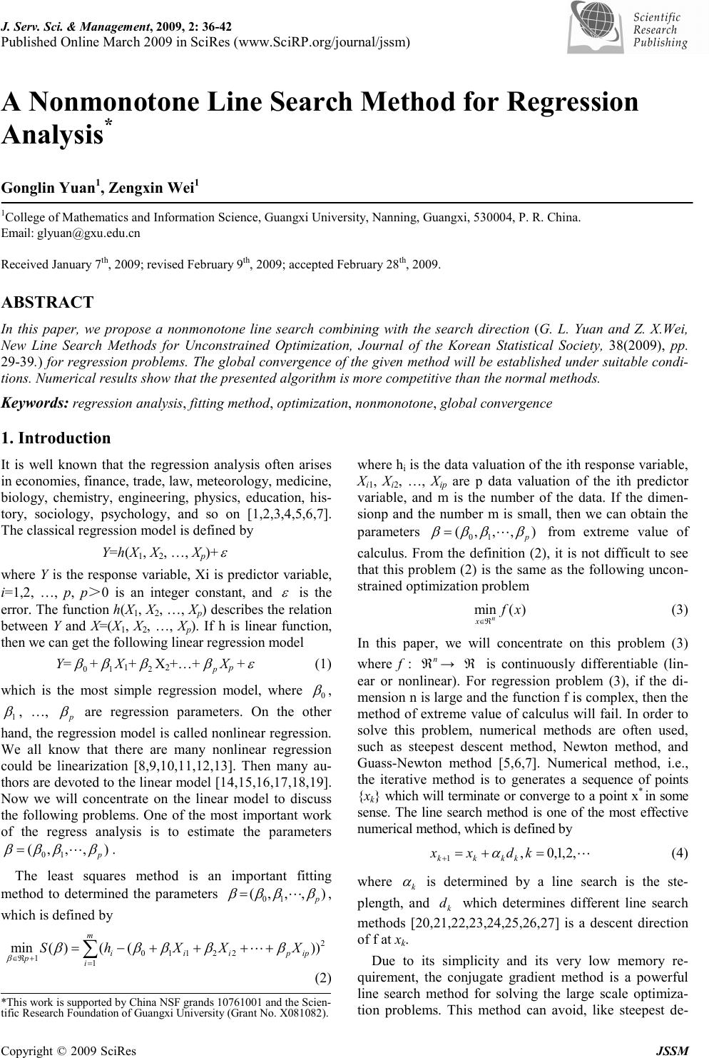J. Serv. Sci. & Management, 2009, 2: 36-42
Published Online March 2009 in SciRes (www.SciRP.org/journal/jssm)
A Nonmonotone Line Search Method for Regression
Analysis
*
Gonglin Yuan
1
, Zengxin Wei
1
1
College of Mathematics and Information Science, Guangxi University, Nanning, Guangxi, 530004, P. R. China.
Received January 7
th
, 2009; revised February 9
th
, 2009; accepted February 28
th
, 2009.
ABSTRACT
In this paper, we propose a nonmonotone line search combining with the search direction (G. L. Yuan and Z. X.Wei,
New Line Search Methods for Unconstrained Optimization, Journal of the Korean Statistical Society, 38(2009), pp.
29-39.) for regression problems. The global convergence of the given method will be established under suitable condi-
tions. Numerical results show that the presented algorithm is more competitive than the normal methods.
Keywords: regression analysis, fitting method, optimization, nonmonotone, global convergence
1. Introduction
It is well known that the regression analysis often arises
in economies, finance, trade, law, meteorology, medicine,
biology, chemistry, engineering, physics, education, his-
tory, sociology, psychology, and so on [1,2,3,4,5,6,7].
The classical regression model is defined by
Y=h(X
1
, X
2
, …, X
p
)+
ε
where Y is the response variable, Xi is predictor variable,
i=1,2, …, p, p＞0 is an integer constant, and
ε
is the
error. The function h(X
1
, X
2
, …, X
p
) describes the relation
between Y and X=(X
1
, X
2
, …, X
p
). If h is linear function,
then we can get the following linear regression model
Y=
0
β +
1
β X
1
+
2
β X
2
+…+
p
β X
p
+
ε
(1)
which is the most simple regression model, where
0
β ,
1
β , …,
p
β are regression parameters. On the other
hand, the regression model is called nonlinear regression.
We all know that there are many nonlinear regression
could be linearization [8,9,10,11,12,13]. Then many au-
thors are devoted to the linear model [14,15,16,17,18,19].
Now we will concentrate on the linear model to discuss
the following problems. One of the most important work
of the regress analysis is to estimate the parameters
),,,(
10 p
ββββ L=.
The least squares method is an important fitting
method to determined the parameters ),,,(
10 p
ββββ L= ,
which is defined by
∑
=
+ℜ∈
++++−=
m
iippiii
p
XXXhS
1
2
22110
1
))(()(min βββββ
β
L
(2)
where h
i
is the data valuation of the ith response variable,
X
i1
, X
i2
, …, X
ip
are p data valuation of the ith predictor
variable, and m is the number of the data. If the dimen-
sionp and the number m is small, then we can obtain the
parameters ),,,(
10 p
ββββ L= from extreme value of
calculus. From the definition (2), it is not difficult to see
that this problem (2) is the same as the following uncon-
strained optimization problem
)(min xf
n
xℜ∈
(3)
In this paper, we will concentrate on this problem (3)
where f :
n
ℜ →
ℜ
is continuously differentiable (lin-
ear or nonlinear). For regression problem (3), if the di-
mension n is large and the function f is complex, then the
method of extreme value of calculus will fail. In order to
solve this problem, numerical methods are often used,
such as steepest descent method, Newton method, and
Guass-Newton method [5,6,7]. Numerical method, i.e.,
the iterative method is to generates a sequence of points
{x
k
} which will terminate or converge to a point x
*
in some
sense. The line search method is one of the most effective
numerical method, which is defined by
L,2,1,0,
1
=+=
+
kdxx
kkkk
α (4)
where
k
α is determined by a line search is the ste-
plength, and
k
d which determines different line search
methods [20,21,22,23,24,25,26,27] is a descent direction
of f at x
k
.
Due to its simplicity and its very low memory re-
quirement, the conjugate gradient method is a powerful
line search method for solving the large scale optimiza-
tion problems. This method can avoid, like steepest de-
*This work is supported by China NSF grands 10761001 and the Scien-
tific Research Foundation of Guangxi University (Grant No. X081082).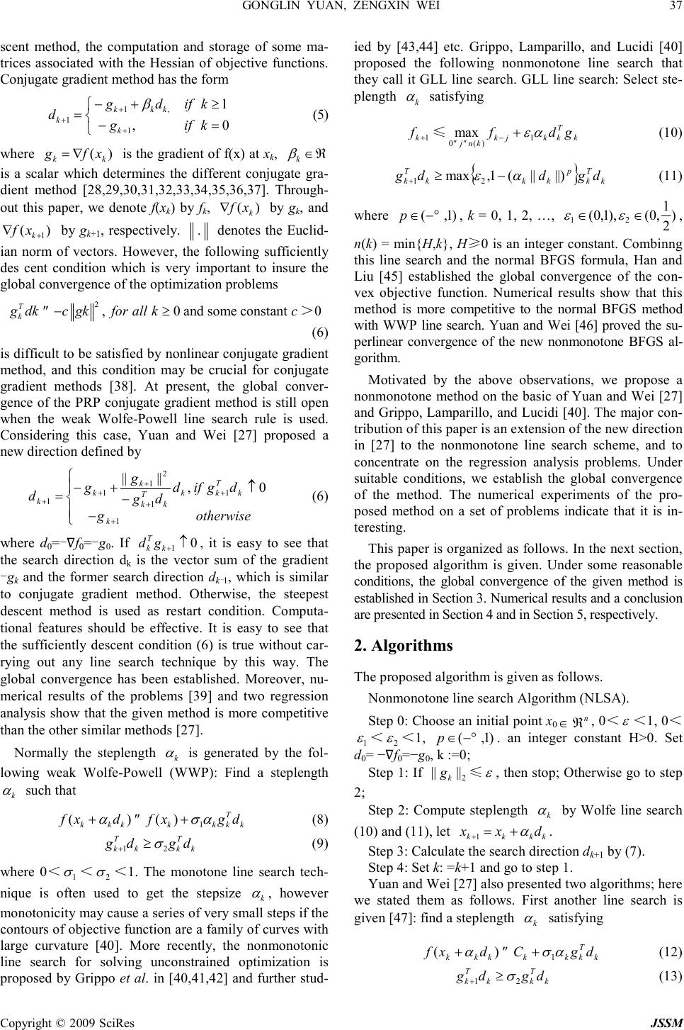

GONGLIN YUAN, ZENGXIN WEI 37
scent method, the computation and storage of some ma-
trices associated with the Hessian of objective functions.
Conjugate gradient method has the form



=−
≥+−
=
+
+
+
0,
1
1
,1
1
kifg
kifdg
d
k
kkk
k
β
(5)
where )(
kk
xfg ∇= is the gradient of f(x) at x
k
, ℜ∈
k
β
is a scalar which determines the different conjugate gra-
dient method [28,29,30,31,32,33,34,35,36,37]. Through-
out this paper, we denote f(x
k
) by f
k
, )(
k
xf∇
by g
k
, and
)(
1+
∇
k
xf by g
k+1
, respectively. . denotes the Euclid-
ian norm of vectors. However, the following sufficiently
des cent condition which is very important to insure the
global convergence of the optimization problems
2
,0 and some constant
T
k
gdkcgkfor all kc
≤ −≥ ＞0
(6)
is difficult to be satisfied by nonlinear conjugate gradient
method, and this condition may be crucial for conjugate
gradient methods [38]. At present, the global conver-
gence of the PRP conjugate gradient method is still open
when the weak Wolfe-Powell line search rule is used.
Considering this case, Yuan and Wei [27] proposed a
new direction defined by





−
≠
−
+−
=
+
+
+
+
+
+
otherwiseg
dgifd
dg
g
g
d
k
k
T
kk
k
T
k
k
k
k
1
1
1
2
1
1
1
0,
||||
(6)
where d
0
=-∇f
0
=-g
0
. If 0
1
≠
+k
T
k
gd , it is easy to see that
the search direction d
k
is the vector sum of the gradient
- g
k
and the former search direction d
k
-
1
, which is similar
to conjugate gradient method. Otherwise, the steepest
descent method is used as restart condition. Computa-
tional features should be effective. It is easy to see that
the sufficiently descent condition (6) is true without car-
rying out any line search technique by this way. The
global convergence has been established. Moreover, nu-
merical results of the problems [39] and two regression
analysis show that the given method is more competitive
than the other similar methods [27].
Normally the steplength
k
α is generated by the fol-
lowing weak Wolfe-Powell (WWP): Find a steplength
k
α such that
k
T
kkkkkk
dgxfdxf ασα
1
)()(+≤+ (8)
k
T
kk
T
k
dgdg
21
σ ≥
+
(9)
where 0 ＜
1
σ ＜
2
σ ＜ 1. The monotone line search tech-
nique is often used to get the stepsize
k
α , however
monotonicity may cause a series of very small steps if the
contours of objective function are a family of curves with
large curvature [40]. More recently, the nonmonotonic
line search for solving unconstrained optimization is
proposed by Grippo et al. in [40,41,42] and further stud-
ied by [43,44] etc. Grippo, Lamparillo, and Lucidi [40]
proposed the following nonmonotone line search that
they call it GLL line search. GLL line search: Select ste-
plength
k
α satisfying
1+k
f ≤
k
T
kkjk
knj
gdf αε
1
)(0
max +
−
≤≤
(10)
{
}
k
T
k
p
kkk
T
k
dgddg ||)||(1,max
21
αε −≥
+
(11)
where )1,(−∞∈p , k = 0, 1, 2, …, )
2
1
,0(),1,0(
21
∈∈ εε ,
n(k) = min{H,k}, H ≥ 0 is an integer constant. Combinng
this line search and the normal BFGS formula, Han and
Liu [45] established the global convergence of the con-
vex objective function. Numerical results show that this
method is more competitive to the normal BFGS method
with WWP line search. Yuan and Wei [46] proved the su-
perlinear convergence of the new nonmonotone BFGS al-
gorithm.
Motivated by the above observations, we propose a
nonmonotone method on the basic of Yuan and Wei [27]
and Grippo, Lamparillo, and Lucidi [40]. The major con-
tribution of this paper is an extension of the new direction
in [27] to the nonmonotone line search scheme, and to
concentrate on the regression analysis problems. Under
suitable conditions, we establish the global convergence
of the method. The numerical experiments of the pro-
posed method on a set of problems indicate that it is in-
teresting.
This paper is organized as follows. In the next section,
the proposed algorithm is given. Under some reasonable
conditions, the global convergence of the given method is
established in Section 3. Numerical results and a conclusion
are presented in Section 4 and in Section 5, respectively.
2. Algorithms
The proposed algorithm is given as follows.
Nonmonotone line search Algorithm (NLSA).
Step 0: Choose an initial point x
0
∈
n
ℜ
, 0 ＜
ε
＜ 1, 0 ＜
1
ε ＜
2
ε ＜ 1, )1,(−∞∈p . an integer constant H>0. Set
d
0
= − ∇ f
0
=−g
0
, k :=0;
Step 1: If
2
||||
k
g ≤
ε
, then stop; Otherwise go to step
2; Step 2: Compute steplength
k
α by Wolfe line search
(10) and (11), let
kkkk
dxx α +=
+1
.
Step 3: Calculate the search direction d
k+1
by (7).
Step 4: Set k: =k+1 and go to step 1.
Yuan and Wei [27] also presented two algorithms; here
we stated them as follows. First another line search is
given [47]: find a steplength
k
α satisfying
k
T
kkkkkk
dgCdxf ασα
1
)( +≤+ (12)
k
T
kk
T
k
dgdg
21
σ ≥
+
(13)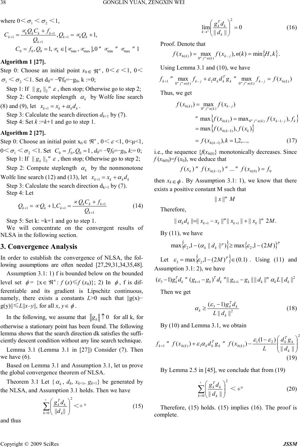

38 GONGLIN YUAN, ZENGXIN WEI
where 0 ＜
1
σ ＜
2
σ ＜ 1,
10],,[,1,
,1,
maxminmaxmin000
1
1
1
1
≤≤≤∈==
+=
+
=
+
+
+
+
µµµµµ
µ
µ
k
kkk
k
kkkk
k
QfC
QQ
Q
fCQ
C
Algorithm 1 [27].
Step 0: Choose an initial point x
0
∈
n
ℜ
, 0 ＜
ε
＜ 1, 0 ＜
1
σ ＜
2
σ ＜ 1. Set d
0
= − ∇ f
0
=−g
0
, k :=0;
Step 1: If ε ≤
2
||||
k
g , then stop; Otherwise go to step 2;
Step 2: Compute steplength
k
α by Wolfe line search
(8) and (9), let
kkkk
dxx α +=
+1
.
Step 3: Calculate the search direction d
k+1
by (7).
Step 4: Set k :=k+1 and go to step 1.
Algorithm 2 [27].
Step 0: Choose an initial point x
0
∈
n
ℜ , 0 ＜
ε
<1, 0< µ <1,
0 ＜
1
σ ＜
2
σ ＜ 1. Set 1,
000
==QfC , d
0
= − ∇ f
0
=−g
0
, k:= 0;
Step 1: If ε ≤
2
||||
k
g , then stop; Otherwise go to step 2;
Step 2: Compute steplength
k
α by the nonmonotone
Wolfe line search (12) and (13), let
kkkk
dxx α +=
+1
Step 3: Calculate the search direction d
k+1
by (7).
Step 4: Let
1
1
11
,1
+
+
++
+
=+=
k
kkk
kkk
Q
fCQ
CQQ
µ
µ (14)
Step 5: Set k: =k+1 and go to step 1.
We will concentrate on the convergent results of
NLSA in the following section.
3. Convergence Analysis
In order to establish the convergence of NLSA, the fol-
lowing assumptions are often needed [27,29,31,34,35,48].
Assumption 3.1: 1) f is bounded below on the bounded
level set
φ
= {x
∈
n
ℜ : f (x) ≤ f (x
0
)}; 2) In
φ
, f is dif-
ferentiable and its gradient is Lipschitz continuous,
namely, there exists a constants L>0 such that ||g(x)−
g(y)|| ≤ L||x–y||, for all x, y
∈
φ
.
In the following, we assume that 0≠
k
g for all k, for
otherwise a stationary point has been found. The following
lemma shows that the search direction dk satisfies the suffi-
ciently descent condition without any line search technique.
Lemma 3.1 (Lemma 3.1 in [27]) Consider (7). Then
we have (6).
Based on Lemma 3.1 and Assumption 3.1, let us prove
the global convergence theorem of NLSA.
Theorem 3.1 Let {
k
α , d
k
, x
k+1
, g
k+1
} be generated by
the NLSA, and Assumption 3.1 holds. Then we have
2
0
||||
∑
∞
=








kk
k
T
k
d
dg
＜ +
∞
(15)
and thus
0
||||
lim
2
=








∞→ k
k
T
k
k
d
dg
(16)
Proof. Denote that
{
}
kHknxfxf
jk
knj
kh
,min)(),(max)(
)(0
)(
==
−
≤≤
.
Using Lemma 3.1 and (10), we have
)(maxmax
)(
)(0
1
)(0
1khjk
knj
k
T
kkjk
knj
k
xffgdff =≤+≤
−
≤≤
−
≤≤
+
αε
Thus, we get
)(max)(
)(0
)( jk
knj
kh
xfxf
−
≤≤
=
{
}
kjkknjkh
fxfxf ),(max)(max
1)(0)( −−≤≤
=≤
{
}
)(),(max
)1( kkh
xfxf
−
=
,...,2,1),(
)1(
==
−
kxf
kh
(17)
i.e., the sequence {f(x
h(k)
} monotonically decreases. Since
f (x
h(0)
)=f (x
0
), we deduce that
0)0()1(
)(...)()( fxfxfxf
hkhk
=≤≤≤
−
then x
k
φ
∈
. By Assumption 3.1: 1), we know that there
exists a positive constant M such that
Mx ≤||||
Therefore,
.2||||||||||||||||
11
Mxxxxd
kkkkkk
≤+≤−=
++
α
By (11), we have
{
}
{
}
P
p
kk
Md )2(1,max)||||(1,max
22
−≥− εαε
Let
{
}
)1.0()2(1,max
23
∈−=
P
M εε . Using (11) and
Assumption 3.1: 2), we have
2
113
||||||||||||)()1(
kkkkkk
T
kkk
T
k
dLdggdggdg αε ≤−≤−≤−
++
Then we get
2
3
||||
)1(
k
k
T
k
k
dL
dg−
≥
ε
α (18)
By (10) and Lemma 3.1, we obtain
2
21
)(1)(1
||||
)1(
)()( 







−
−≤+≤
+
k
k
T
k
khk
T
kkkhk
d
gd
L
xfgdxff
εε
αε
(19)
By Lemma 2.5 in [45], we conclude that from (19)
∑
∞
=








0
2
||||
kk
k
T
k
d
dg
＜
+∞
(20)
Therefore, (15) holds. (15) implies (16). The proof is
complete.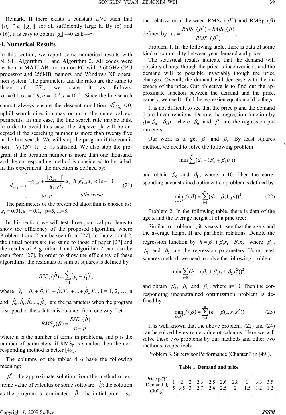

GONGLIN YUAN, ZENGXIN WEI 39
Remark. If there exists a constant c
0
>0 such that
||||||||
0kk
gcd ≤ for all sufficiently large k. By (6) and
(16), it is easy to obtain ||g
k
|| → 0 as k →∞ .
4. Numerical Results
In this section, we report some numerical results with
NLST, Algorithm 1, and Algorithm 2. All codes were
written in MATLAB and run on PC with 2.60GHz CPU
processor and 256MB memory and Windows XP opera-
tion system. The parameters and the rules are the same to
those of [27], we state it as follows:
54
21
10,10,9.0,1.0
−−
==== εµσσ . Since the line search
cannot always ensure the descent condition
k
T
k
gd ＜ 0,
uphill search direction may occur in the numerical ex-
periments. In this case, the line search rule maybe fails.
In order to avoid this case, the stepsize _k will be ac-
cepted if the searching number is more than twenty five
in the line search. We will stop the program if the condi-
tion 51||)(|| −∇ef β is satisfied. We also stop the pro-
gram if the iteration number is more than one thousand,
and the corresponding method is considered to be failed.
In this experiment, the direction is defined by:
2
1
1 1
11
1
1 10
,
|| ||
,
T
k
kkk k
T
kk k
k
g
gdif gde
dg d
g otherwise
+
+ +
++
+

−+< −

=−

−

(21)
The parameters of the presented algorithm is chosen as:
,1.0,01.0
21
== εε p=5, H=8.
In this section, we will test three practical problems to
show the efficiency of the proposed algorithm, where
Problem 1 and 2 can be seen from [27]. In Table 1 and 2,
the initial points are the same to those of paper [27] and
the results of Algorithm 1 and Algorithm 2 can also be
seen from [27]. In order to show the efficiency of these
algorithms, the residuals of sum of squares is defined by
( )
∑
=
−=
n
iip
yySSE
1
2
1
,
ˆ
)
ˆ
( β
where ,
ˆ
...
ˆˆˆ
ˆ
221101 ippii
XXXy ββββ ++++= i = 1, 2, …, n,
and
p
ββββ
ˆ
,...,
ˆ
,
ˆ
,
ˆ
210
are the parameters when the program
is stopped or the solution is obtained from one way. Let
pn
SSE
RMS
p
p
−
=)
ˆ
(
)
ˆ
(
β
β
where n is the number of terms in problems, and p is the
number of parameters, if RMS
p
is smaller, then the cor-
responding method is better [49].
The columns of the tables 4 - 6 have the following
meaning:
*
β : the approximate solution from the method of ex-
treme value of calculus or some software. : the solution
as the program is terminated. β
(
: the initial point.
*
ε :
the relative error between RMS
p
(
*
β ) and RMSp ()
defined by
)(
)()(
*
*
*
β
ββ
ε
p
pp
RMS
RMSRMS −
= .
Problem 1. In the following table, there is data of some
kind of commodity between year demand and price:
The statistical results indicate that the demand will
possibly change though the price is inconvenient, and the
demand will be possible invariably though the price
changes. Overall, the demand will decrease with the in-
crease of the price. Our objective is to find out the ap-
proximate function between the demand and the price,
namely, we need to find the regression equation of d to the p.
It is not difficult to see that the price p and the demand
d are linear relations. Denote the regression function by
p
10
ββ += , where
0
β and
1
β are the regression pa-
rameters.
Our work is to get
0
β and
1
β . By least squares
method, we need to solve the following problem
∑
=
+−
n
iii
pd
0
2
10
))((min ββ
and obtain
0
β and
1
β , where n=10. Then the corre-
sponding unconstrained optimization problem is defined by
∑
=
∈
−=
n
iii
R
pdf
1
2
)),1(()(min
2
ββ
β
(22)
Problem 2. In the following table, there is data of the
age x and the average height H of a pine tree:
Similar to problem 1, it is easy to see that the age x and
the average height H are parabola relations. Denote the
regression function by
22110
ˆxxh
βββ ++= , where
0
β ,
1
β and
2
β are the regression parameters. Using least
squares method, we need to solve the following problem
∑
=
++−
n
iiii
xxh
0
22
210
))((min βββ
and obtain
0
β ,
1
β and
2
β , where n=10. Then the cor-
responding unconstrained optimization problem is de-
fined by
∑
=
∈
−=
n
iiii
R
xxhf
1
22
,
)),1(()(min
3
ββ
β
(23)
It is well known that the above problems (22) and (24)
can be solved by extreme value of calculus. Here we will
solve these two problems by our methods and other two
methods, respectively.
Problem 3. Supervisor Performance (Chapter 3 in [49]).
Table 1. Demand and price
Price p
i
($)
Demand d
i
(500g)
1
5
2
3.5
2
3
2.3
2.7
2.5
2.4
2.6
2.5
2.8
2
3
1.5
3.3
1.2
3.5
1.2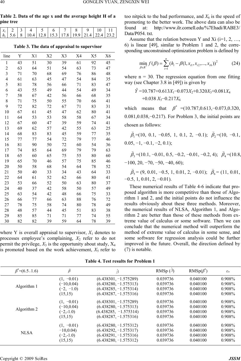

40 GONGLIN YUAN, ZENGXIN WEI
Table 2. Data of the age x and the average height H of a
pine tree
x
i
h
i
2
5.6
3
8
4
10.4
5
12.8
6
15.3
7
17.8
8
19.9
9
21.4
10
22.4
11
23.2
Table 3. The data of appraisal to supervisor
line Y X1 X2 X3 X4 X5 X6
1 43 51 30 39 61 92 45
2 63 64 51 54 63 73 47
3 71 70 68 69 76 86 48
4 61 63 45 47 54 84 35
5 81 78 56 66 71 83 47
6 43 55 49 44 54 49 34
7 58 67 42 56 66 68 35
8 71 75 50 55 70 66 41
9 72 82 72 67 71 83 31
10 67 61 45 47 62 80 41
11 64 53 53 58 58 67 34
12 67 60 47 39 59 74 41
13 69 62 57 42 55 63 25
14 68 83 83 45 59 77 35
15 77 77 54 72 79 77 46
16 81 90 50 72 60 54 36
17 74 85 64 69 79 79 63
18 65 60 65 75 55 80 60
19 65 70 46 57 75 85 46
20 50 58 68 54 64 78 52
21 50 40 33 34 43 64 33
22 64 61 52 62 66 80 41
23 53 66 52 50 63 80 37
24 40 37 42 58 50 57 49
25 63 54 42 48 66 75 33
26 66 77 66 63 88 76 72
27 78 75 58 74 80 78 49
28 48 57 44 45 51 83 38
29 85 85 71 71 77 74 55
30 82 82 39 59 64 78 39
where Y is overall appraisal to supervisor, X
1
denotes to
processes employee’s complaining, X
2
refer to do not
permit the privilege, X
3
is the opportunity about study, X
4
is promoted based on the work achievement, X
5
refer to
too nitpick to the bad performance, and X
6
is the speed of
promoting to the better work. The above data can also be
found at: http://www.ilr.cornell.edu/%7Ehadi/RABE3/
Data/P054. txt.
Assume that the relation between Y and Xi (i=1, 2, …,
6) is linear [49], similar to Problem 1 and 2, the corre-
sponding unconstrained optimization problem is defined by
∑
=
∈
−=
n
iiiii
R
xxxhf
1
2
621
)),...,,,1(()(min
7
ββ
β
(24)
where n = 30. The regression equation from one fitting
way (see Chapter 3.8 in [49]) is given by
Y
ˆ=10.787+0.613X
1
−0.073X
2
+0.320X
3
+0.081X
4
+0.038 X
5
−0.217X
6
which means that
*
β =(10.787,0.613,−0.073,0.320,
0.081,0.038,−0.217). For Problem 3, the initial points are
chosen as follows:
1
β
(
=(10, 0.1, −0.05, 1, 0.1, 2, −0.1);
2
β
(
=(10, −0.1,
0.05, −1, −0.1, −2, 0.1);
3
β
(
=(10.1, −0.01, 0.5, −0.2, −0.01, −0.2, 4);
4
β
(
=(10.8,
−100, 20, −70, −50, −40, 60);
5
β
(
= (9, 0.01, −0.5, 1, 0.01, 2, −0.01);
6
β
(
= (11, 0.01,
−0.5, 1, 0.01, 2, −0.01).
These numerical results of Table 4-6 indicate that pro-
posed algorithm is more competitive than those of Algo-
rithm 1 and 2, and the initial points do not influence the
results obviously about these three methods. Moreover,
the numerical results of NLSA, Algorithm 1, and Algo-
rithm 2 are better than those of these methods from ex-
treme value of calculus or some software. Then we can
conclude that the numerical method will outperform the
method of extreme value of calculus in some sense, and
some software for regression analysis could be further
improved in the future. Overall, the direction defined by
(7) is notable.
Table 4. Test results for Problem 1
β
*
=(6.5-1.6)
β
(
RMSp () RMSp(β
*
) ε
*
Algorithm 1
(1, -0.01)
(-10,0.04)
(-2, -1.0)
(15,15)
(6.438301, -1.575289)
(6.438280, -1.575313)
(6.438285, -1.575314)
(6.438287, -1.575316)
0.039736
0.039736
0.039736
0.039736
0.040100
0.040100
0.040100
0.040100
0.908%
0.908%
0.908%
0.908%
Algorithm 2
(1, -0.01)
(-10,0.04)
(-2,-1.0)
(15,15)
(6.438301, -1.575289)
(6.438280, -1.575313)
(6.438285, -1.575314)
(6.438287, -1.575316)
0.039736
0.039736
0.039736
0.039736
0.040100
0.040100
0.040100
0.040100
0.908%
0.908%
0.908%
0.908%
NLSA
(1, -0.01)
-10,0.04)
(-2,-1.0)
(15,15)
(6.438280, -1.575312)
(6.438292, -1.575317)
(6.438291, -1.575316)
(6.438280, -1.575312)
0.039736
0.039736
0.039736
0.039736
0.040100
0.040100
0.040100
0.040100
0.908%
0.908%
0.908%
0.908%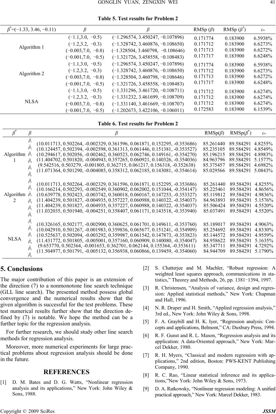

GONGLIN YUAN, ZENGXIN WEI 41
Table 5. Test results for Problem 2
β
*
=(−1.33, 3.46, −0.11) β β RMSp (β) RMSp (β
*
) ε
*
Algorithm 1
(-1.1,3.0, -0.5)
(-1.2,3.2, -0.3)
(-0.003,7.0, -0.8)
(-0.001,7.0, -0.5)
(-1.296574, 3.450247, -0.107896)
(-1.328742, 3.460876, -0.108650)
(-1.328504, 3.460798, -0.108646)
(-1.321726, 3.458558, -0.108483)
0.171774
0.171712
0.171713
0.171717
0.183900
0.183900
0.183900
0.183900
6.5938%
6.6273%
6.6272%
6.6248%
Algorithm 2
(-1.1,3.0, -0.5)
(-1.2,3.2, -0.3)
(-0.003,7.0, -0.8)
(-0.001,7.0, -0.5)
(-1.296574, 3.450247, -0.107896)
(-1.328742, 3.460876, -0.108650)
(-1.328504, 3.460798, -0.108646)
(-1.321726, 3.458558, -0.108483)
0.171774
0.171712
0.171713
0.171717
0.183900
0.183900
0.183900
0.183900
6.5938%
6.6273%
6.6272%
6.6248%
NLSA
(-1.1,3.0, -0.5)
(-1.2,3.2, -0.3)
(-0.003,7.0, -0.8)
(-0.001,7.0, -0.5)
(-1.331296, 3.461720, -0.108711)
(-1.331232, 3.461699, -0.108709)
(-1.331140, 3.461669, -0.108707)
(-1.202673, 3.422106, -0.106011)
0.171712
0.171712
0.171712
0.172583
0.183900
0.183900
0.183900
0.183900
6.6274%
6.6274%
6.6274%
6.1539%
Table 6. Test results for Problem 2
β
*
β β RMSp(β) RMSp(β
*
) ε
*
Algorithm
1
1
β
(
2
β
(
3
β
(
4
β
(
5
β
(
6
β
(
(10.011713, 0.502264, -0.002329, 0.361596, 0.061871, 0.152295, -0.353686)
(10.124457, 0.502394, -0.002598, 0.361313, 0.061446, 0.151381, -0.353527)
(10.294617, 0.502056, -0.002462, 0.360523, 0.062746, 0.149161, -0.354270)
(11.404702, 0.501820, -0.004943, 0.357265, 0.060921, 0.140326, -0.354036)
(9.542516, 0.503279, -0.001805, 0.362715, 0.061217, 0.156318, -0.352638)
(11.071364, 0.501290, -0.004085, 0.358312, 0.062185, 0.143081, -0.354614)
85.261440
85.235105
85.196215
84.963796
85.375457
85.029566
89.584291
89.584291
89.584291
89.584291
89.584291
89.584291
4.8255%
4.8549%
4.8983%
5.1577%
4.6982%
5.0843%
Algorithm
2
1
β
(
2
β
(
3
β
(
4
β
(
5
β
(
6
β
(
(10.011713, 0.502264, -0.002329, 0.361596, 0.061871, 0.152295, -0.353686)
(10.166214, 0.502293, -0.002549, 0.360902, 0.062002, 0.151044, -0.354147)
(10.639778, 0.502423, -0.003742, 0.360018, 0.060167, 0.147253, -0.353327)
(11.404239, 0.501827, -0.004935, 0.357227, 0.060988, 0.140322, -0.354037)
(11.404239, 0.501827, -0.004935, 0.357227, 0.060988, 0.140322, -0.354037)
(11.032035, 0.501940, -0.004251, 0.358407, 0.061171, 0.143518, -0.353940)
85.261440
85.225461
85.119812
84.963893
85.506424
85.037491
89.584291
89.584291
89.584291
89.584291
89.584291
89.584291
4.8255%
4.8656%
4.9836%
5.1576%
4.5520%
4.5520%
NLSA
1
β
(
2
β
(
3
β
(
4
β
(
5
β
(
6
β
(
(10.326165, 0.502177, -0.002900, 0.360625, 0.061701, 0.149611, -0.353760)
(10.042910, 0.501267, -0.001983, 0.359836, 0.065677, 0.151241, -0.354909)
(10.525637, 0.502094, -0.003292, 0.359987, 0.061542, 0.147873, -0.353823)
(11.431772, 0.501805, -0.005001, 0.357160, 0.060909, 0.140080, -0.354047)
(9.653770, 0.502364, -0.001653, 0.362701, 0.062144, 0.155364, -0.353611)
(11.504977, 0.501791, -0.005132, 0.356938, 0.060866, 0.139459, -0.354060)
85.189017
85.254692
85.144572
84.958622
85.347711
84.944709
89.584291
89.584291
89.584291
89.584291
89.584291
89.584291
4.9063%
4.8330%
4.9559%
5.1635%
4.7292%
5.1790%
5. Conclusions
The major contribution of this paper is an extension of
the direction (7) to a nonmonotone line search technique
(GLL line search). The presented method possess global
convergence and the numerical results show that the
given algorithm is successful for the test problems. These
test numerical results further show that the direction de-
fined by (7) is notable. We hope the method can be a
further topic for the regression analysis.
For further research, we should study other line search
methods for regression analysis.
Moreover, more numerical experiments for large prac-
tical problems about regression analysis should be done
in the future.
REFERENCES
[1] D. M. Bates and D. G. Watts, “Nonlinear regression
analysis and its applications,” New York: John Wiley &
Sons, 1988.
[2] S. Chatterjee and M. Machler, “Robust regression: A
weighted least squares approach, communications in sta-
tistics,” Theorey and Methods, 26, pp. 1381-1394, 1997.
[3] R. Christensen, “Analysis of variance, design and regres-
sion: Applied statistical methods,” New York: Chapman
and Hall, 1996.
[4] N. R. Draper and H. Smith, “Applied regression analysis,”
3rd ed., New York: John Wiley & Sons, 1998.
[5] F. A. Graybill and H. K. Iyer, “Regression analysis: Con-
cepts and applications, Belmont,” CA: Duxbury Press, 1994.
[6] R. F. Gunst and R. L. Mason, “Regression analysis and its
application: A data-Oriented approach,” New York: Mar-
cel Dekker, 1980.
[7] R. H. Myers, “Classical and modern regression with ap-
plications,” 2nd edition, Boston: PWS-KENT Publishing
Company, 1990.
[8] R. C. Rao, “Linear statistical inference and its applica-
tions,”New York: John Wiley & Sons, 1973.
[9] D. A. Ratkowsky, “Nonlinear regression modeling: A unified
practical approach,” New York: Marcel Dekker, 1983.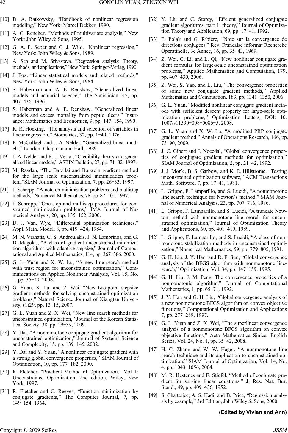

42 GONGLIN YUAN, ZENGXIN WEI
[10] D. A. Ratkowsky, “Handbook of nonlinear regression
modeling,” New York: Marcel Dekker, 1990.
[11] A. C. Rencher, “Methods of multivariate analysis,” New
York: John Wiley & Sons, 1995.
[12] G. A. F. Seber and C. J. Wild, “Nonlinear regression,”
New York: John Wiley & Sons, 1989.
[13] A. Sen and M. Srivastava, “Regression analysis: Theory,
methods, and applications,” New York: Springer-Verlag, 1990.
[14] J. Fox, “Linear statistical models and related methods,”
New York: John Wiley & Sons, 1984.
[15] S. Haberman and A. E. Renshaw, “Generalized linear
models and actuarial science,” The Statistician, 45, pp.
407-436, 1996.
[16] S. Haberman and A. E. Renshaw, “Generalized linear
models and excess mortality from peptic ulcers,” Insur-
ance: Mathematics and Economics, 9, pp. 147-154, 1990.
[17] R. R. Hocking, “The analysis and selection of variables in
linear regression,” Biometrics, 32, pp. 1-49, 1976.
[18] P. McCullagh and J. A. Nelder, “Generalized linear mod-
els,” London: Chapman and Hall, 1989.
[19] J. A. Nelder and R. J. Verral, “Credibility theory and gener-
alized linear models,” ASTIN Bulletin, 27, pp. 71-82, 1997.
[20] M. Raydan, “The Barzilai and Borwein gradient method
for the large scale unconstrained minimization prob-
lem,”SIAM Journal of Optimization, 7, pp. 26-33, 1997.
[21] J. Schropp, “A note on minimization problems and multistep
methods,” Numerical Mathematics, 78, pp. 87-101, 1997.
[22] J. Schropp, “One-step and multistep procedures for con-
strained minimization problems,” IMA Journal of Nu-
merical Analysis, 20, pp. 135-152, 2000.
[23] D. J. Van. Wyk, “Differential optimization techniques,”
Appl. Math. Model, 8, pp. 419-424, 1984.
[24] M. N. Vrahatis, G. S. Androulakis, J. N. Lambrinos, and G.
D. Magolas, “A class of gradient unconstrained minimiza-
tion algorithms with adaptive stepsize,” Journal of Compu-
tational and Applied Mathematics, 114, pp. 367-386, 2000.
[25] G. L. Yuan and X. W. Lu, “A new line search method
with trust region for unconstrained optimization,” Com-
munications on Applied Nonlinear Analysis, Vol. 15, No.
1, pp. 35-49, 2008.
[26] G. Yuan, X. Lu, and Z. Wei, “New two-point stepsize
gradient methods for solving unconstrained optimization
problems,” Natural Science Journal of Xiangtan Univer-
sity, (1)29, pp. 13-15, 2007.
[27] G. L. Yuan and Z. X. Wei, “New line search methods for
unconstrained optimization,” Journal of the Korean Statis-
tical Society, 38, pp. 29-39, 2009.
[28] Y. Dai, “A nonmonotone conjugate gradient algorithm for
unconstrained optimization,” Journal of Systems Science
and Complexity, 15, pp. 139-145, 2002.
[29] Y. Dai and Y. Yuan, “A nonlinear conjugate gradient with
a strong global convergence properties,” SIAM Journal of
Optimization, 10, pp. 177-182, 2000.
[30] R. Fletcher, “Practical Method of Optimization,” Vol 1:
Unconstrained Optimization, 2nd edition, Wiley, New
York, 1997.
[31] R. Fletcher and C. Reeves, “Function minimization by
conjugate gradients,” The Computer Journal, 7, pp,
149-154, 1964.
[32] Y. Liu and C. Storey, “Effcient generalized conjugate
gradient algorithms, part 1: theory,” Journal of Optimiza-
tion Theory and Application, 69, pp. 17-41, 1992.
[33] E. Polak and G. Ribiere, “Note sur la convergence de
directions conjugees,” Rev. Francaise informat Recherche
Operatinelle, 3e Annee, 16, pp. 35-43, 1969.
[34] Z. Wei, G. Li, and L. Qi, “New nonlinear conjugate gra-
dient formulas for large-scale unconstrained optimization
problems,” Applied Mathematics and Computation, 179,
pp. 407-430, 2006.
[35] Z. Wei, S. Yao, and L. Liu, “The convergence properties
of some new conjugate gradient methods,” Applied
Mathematics and Computation, 183, pp. 1341-1350, 2006.
[36] G. L. Yuan, “Modified nonlinear conjugate gradient meth-
ods with sufficient descent property for large-scale opti-
mization problems,” Optimization Letters, DOI: 10.
1007/s11590-008-0086-5, 2008.
[37] G. L. Yuan and X. W. Lu, “A modified PRP conjugate
gradient method,” Annals of Operations Research, 166, pp.
73-90, 2009.
[38] J. C. Gibert and J. Nocedal, “Global convergence proper-
ties of conjugate gradient methods for optimization,”
SIAM Journal of Optimization, 2, pp. 21-42, 1992.
[39] J. J. Mor´e, B. S. Garbow, and K. E. Hillstrome, “Testing
unconstrained optimization software,” ACM Transactions
Math. Software, 7, pp. 17-41, 1981.
[40] L. Grippo, F. Lamparillo, and S. Lucidi, “A nonmonotone
line search technique for Newton’s method,” SIAM Jour-
nal of Numerical Analysis, 23, pp. 707-716, 1986.
[41] L. Grippo, F. Lamparillo, and S. Lucidi, “A truncate New-
ton method with nonmonotone line search for uncon-
strained optimization,” Journal of Optimization Theory
and Applications, 60, pp. 401-419, 1989.
[42] L. Grippo, F. Lamparillo, and S. Lucidi, “A class of non-
monotone stabilization methods in unconstrained optimi-
zation,” Numerical Mathematics, 59, pp. 779-805, 1991.
[43] G. H. Liu, J. Y. Han, and D. F. Sun, “Global convergence
analysis of the BFGS algorithm with nonmonotone line-
search,” Optimization, Vol. 34, pp. 147-159, 1995.
[44] G. H. Liu, J. M. Peng, The convergence properties of a
nonmonotonic algorithm,” Journal of Computational
Mathematics, 1, pp. 65-71, 1992.
[45] J. Y. Han and G. H. Liu, “Global convergence analysis of
a new nonmonotone BFGS algorithm on convex objective
functions,” Computational Optimization and Applications
7, pp. 277-289, 1997.
[46] G. L. Yuan and Z. X. Wei, “The superlinear convergence
analysis of a nonmonotone BFGS algorithm on convex
objective functions,” Acta Mathematica Sinica, English
Series, Vol. 24, No. 1, pp. 35-42, 2008.
[47] H. C. Zhang and W. W. Hager, “A nonmonotone line
search technique and its application to unconstrained op-
timization,” SIAM Journal of Optimization, Vol. 14, No.
4, pp. 1043-1056, 2004.
[48] M. R. Hestenes and E. Stiefel, “Method of conjugate gra-
dient for solving linear equations,” J, Res. Nat. Bur.
Stand., 49, pp. 409-436, 1952.
[49] S. Chatterjee, A. S. Hadi, and B. Price, “Regression analy-
sis by example,” 3rd Edition, John Wiley & Sons, 2000.
(Edited by Vivian and Ann)