Circuits and Systems
Vol.07 No.09(2016), Article ID:68630,27 pages
10.4236/cs.2016.79206
Ant Lion Optimization Approach for Load Frequency Control of Multi-Area Interconnected Power Systems
R. Satheeshkumar, R. Shivakumar
EEE, Sona College of Technology, Salem, India

Copyright © 2016 by authors and Scientific Research Publishing Inc.
This work is licensed under the Creative Commons Attribution International License (CC BY).
http://creativecommons.org/licenses/by/4.0/


Received 24 March 2016; accepted 20 April 2016; published 19 July 2016
ABSTRACT
This work proposes a novel nature-inspired algorithm called Ant Lion Optimizer (ALO). The ALO algorithm mimics the search mechanism of antlions in nature. A time domain based objective function is established to tune the parameters of the PI controller based LFC, which is solved by the proposed ALO algorithm to reach the most convenient solutions. A three-area interconnected power system is investigated as a test system under various loading conditions to confirm the effectiveness of the suggested algorithm. Simulation results are given to show the enhanced performance of the developed ALO algorithm based controllers in comparison with Genetic Algorithm (GA), Particle Swarm Optimization (PSO), Bat Algorithm (BAT) and conventional PI controller. These results represent that the proposed BAT algorithm tuned PI controller offers better performance over other soft computing algorithms in conditions of settling times and several performance indices.
Keywords:
Load Frequency Control (LFC), Multi-Area Power System, Proportional-Integral (PI) Controller, Ant Lion Optimization (ALO), Bat Algorithm (BAT), Genetic Algorithm (GA), Particle Swarm Optimization (PSO)

1. Introduction
Load Frequency Control (LFC) is a crucial topic in power system operation and control of supplying sufficient and dependable electric power with better tone. An electric energy system must be maintained at a desired operating level characterized by nominal frequency and voltage profile, and this is achieved by close control of real and reactive powers generated through the controllable source of the system. The primary destination of the LFC is to maintain zero steady state errors for frequency deviation, and right tracking load demands in a multi-area power system [1] - [4] . During the last decades, many technical papers have been distributed with the LFC in power system literature by using analogy models, such as [5] [6] . In Ref. [5] , an LFC model is considered by using linear feedback. In [6] , a new approach is reported for optimal control of power systems.
In the event of an interconnected power system, any small sudden load change in any of the areas causes the variation of the frequencies of each and every area and likewise at that place is a fluctuation of power in tie line. The primary objective of Load Frequency Control (LFC) area is to maintain the right frequency, besides the desired power output (megawatt) in the interconnected power system and to monitor the change in tie line power between control areas. Thus, an LFC scheme incorporates an appropriate control system for an interconnected power system. It is heaving the capability to bring the frequencies of each area and the tie line powers back to original setpoint values or very nearer to set point values effectively after the load change because of the of conventional controllers. Nevertheless, the conventional controllers are having some demerits like; they are very sluggish in functioning. They do not care about the inherent nonlinearities of different power system components; it is very hard to decide the gain of the integrator setting according to changes in the operating point. The artificial intelligence control system delivers many advantages over the conventional integral controller. They are a lot faster than integrated controllers, and besides they give better stability response than integral controllers. Several control strategies for LFC of power systems have been proposed to maintain the frequency and tie-line power flow at their scheduled power values during normal and distributed conditions. Classical controllers are offered for LFC of power system [7] . Also, various soft computing algorithms based controllers such as GA, PSO, Craziness PSO, Bacterial Foraging Optimization, Differential Evaluation, etc., are applied and found the superiority of the power system [8] - [23] .
In this proposed research work, a new form of multi-area power system with a combination of thermal, hydro and PV sources. A new algorithm proposed for load-frequency control, which can both reduce control time and diminish the value of frequency deviation during the active operation of power systems. By developing of industrial controllers, Proportional-Integral (PI) controllers is still one of the most popular controllers. A new approach addressed for load-frequency control of interconnected three area power systems by using an Ant Lion Optimizer (ALO) algorithm in this paper. The algorithm applied to optimize the PI parameters. Also, to adjust the PI controller, the ITAE is used as a cost function. The ITAE criterion was chosen due to it can determine a healthy weight for error signal in terms of time. This event can reduce settling time in the lowest value and damp fluctuations, quickly [24] . In the proposed method, the Area Control Error (ACE) is also fixed and worked out by the feedback in each area; and therefore, the control action is done to set the ACE in zero value. As a result, frequency and tie power among areas are prevented in the stipulated values.
2. Three Area Interconnected Power System
The system under study consists of three areas. Area one is a thermal non-reheat system, area two is a hydro system, and area three is photovoltaic (PV) system [25] [26] . The detailed designed model of three area power system for load frequency control is shown in Figure 1. The thermal plant has a single stage non-reheat steam turbine, and the hydro plant equipped with an electric governor.
System Modelling
The dynamic model of Load Frequency Control (LFC) for a two-area interconnected power system is presented in this section. Each area of the power system consists of speed governing system, turbine, and generator as shown in Figure 1. Each area has three inputs and two outputs. The inputs are the controller input ∆Pref, load disturbance ∆PD and tie-line power error ∆Ptie. The outputs are the generator frequency ∆f and Area Control Error (ACE) given by equation
 (1)
(1)
where B is the frequency bias parameter.
To simplicity the frequency-domain analyzes, transfer functions are used to model each component of the area. Turbine is represented by the transfer function [27] .

Figure 1. A three area LFC power system model.
Transfer function of the governor is
 (2)
(2)
Transfer function of the steam turbine is
 (3)
(3)
Transfer function of the generator is
 (4)
(4)
where Kp = 1/D and Tp = 2H/fD.
Transfer function of the hydraulic turbine is
 (5)
(5)
The system under investigation consists of three area interconnected power system as shown in Figure 1. The system is widely used in literature is for the design and analysis of automatic load frequency control of interconnected areas [28] [29] . In Figure 1, B1 and B2 are the frequency bias parameters; ACE1, ACE2, and ACE3 are area control errors; u1, u2, and u3 are the control outputs from the controller; R1 and R2 are the governor speed regulation parameters in pu Hz; Tg1 and Tg2 are the speed governor time constants in sec; DPV1 and DPV2 are the change in governor valve positions (pu); DPg1 and DPg2 are the governor output command (p.u). Tt1 and Tt2 are the turbine time constant in sec; DPt1 and DPt2 are the change in turbine output powers; dPD1, dPD2, and dPD3 are the load demand changes; DPTie is the incremental change in tie line power (p.u); KPS1, KPS2, and KPS3 are the power system gains; TPS1, TPS2, and TPS3 are the power system time constant in sec; T12, T23, and T31 are the synchronizing coefficient and Df1, Df2 and Df3 are the system frequency deviations in Hz.
3. Design of Pi for Load Frequency Control System
Despite significant strides in the development of advanced control schemes over the past two decades, the conventional Proportional-Integral (PI) controller and its variants remain an engineer’s preferred choice because of its structural simplicity, reliability, and the favorable ratio between performance and cost. Beyond these benefits, it controllers also offers simplified dynamic modeling, lower user-skill requirements, and minimal development effort, which are issues of substantial importance to engineering practice. As the name suggests, the PI algorithm consists of three basic modes, the proportional mode, and integral mode. A proportional controller has the effect of reducing the rise time, but never eliminates the steady-state error. An integral control has the effect of eliminating the steady-state error, but it may make the transient response worse. The design of PI controller requires determination of the two parameters, Proportional gain (KP) and Integral gain (KI) [27] [29] .
The error inputs to the controllers are the respective area control errors (ACE) are:
 (6)
(6)
 (7)
(7)
 (8)
(8)
The control inputs of the power system u1 and u2 are the outputs of the controllers. The control inputs are obtained as:
 (9)
(9)
 (10)
(10)
 (11)
(11)
In the design of a PI controller, the objective function is first defined based on the desired specifications and constraints. The design of objective function to tune PI controller is based on a performance index that considers the entire closed loop response. Typical output specifications in the time domain are peak overshooting, rise time, settling time, and steady-state error. Four kinds of performance criteria usually considered in the control design are the Integral of Time multiplied Absolute Error (ITAE), Integral of Squared Error (ISE) and Integral of Absolute Error (IAE).
The sum of time multiple absolute errors in ACE is considered as a performance index. Hence, J can be:
 (12)
(12)
 (13)
(13)
 (14)
(14)
where J is the objective function and ,
,  and
and ,
,  is the minimum and maximum value of the control parameters. One more important factor that affects the optimal solution more or less is the range for unknowns. The range of unknowns depends on the type of applications. For the very first execution of the program, a wider solution space can be given and after getting the solution, one can shorten the solution space nearer to the values obtained in the previous iteration. To enhance the system response regarding the settling time and overshoots, it is necessary to modify the above equation. The design process can be formed as the following constrained optimization problem.
4. Ant Lion Optimizer Algorithm
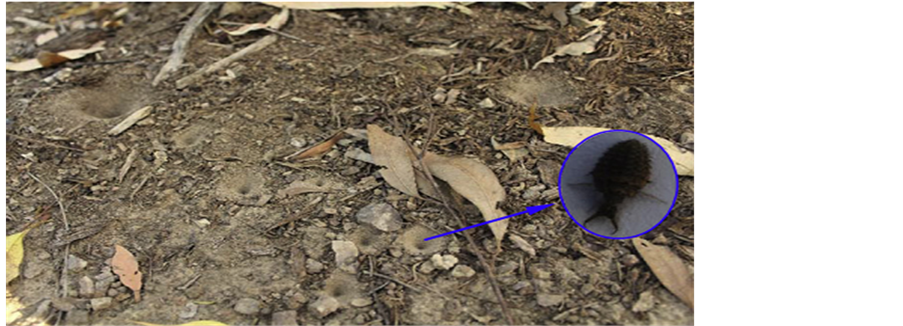
The ALO algorithm also finds superior optimal designs for the majority of classical engineering problems employed, showing that this algorithm has merits in solving constrained problems with separate search spaces. The main inspiration of the ALO algorithm comes from the foraging behavior of antlion’s larvae [30] . Figure 2(a) shows several cone-shaped pits with different sizes. After digging the trap, the larvae hide underneath the bottom of the cone and waits for insects (preferably ant) to be trapped in the pit [30] as illustrated in Figure 2(b). The edge of the cone is sharp enough for insects to fall to the bottom of the trap easily. Once the antlion realizes that prey is in the trap, it tries to catch it.
4.1. Operators of the ALO algorithm
The ALO algorithm mimics interaction between antlions and ants in the trap. To model such interactions, ants are required to move over the search space, and antlions are allowed to hunt them and become fitter using traps. Since ants move stochastically in nature when searching for food, a random walk is chosen for modeling ants’ movement as follows:
 (a)
(a)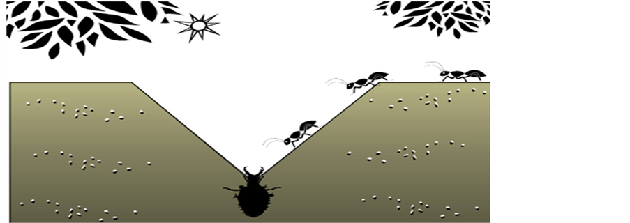 (b)
(b)
Figure 2. Hunting behavior of antlions.
 (15)
(15)
where cumsum calculates the cumulative sum, n is the maximum number of iteration; t shows the step of random walk (iteration in this study), and r(t) is a stochastic function defined as follows:
 (16)
(16)
where t shows the step of random walk (iteration in this study) and rand is a random number generated with uniform distribution in the interval of [0, 1].
Figure 3 shows hunting behavior of antlions. This figure indicates that the random walk utilized may fluctuate dramatically around the origin (red curve), have increasing trend (black curve), or have descending behavior (blue curve).
The position of ants is saved and utilized during optimization in the following matrix:
 (17)
(17)
where MAnt is the matrix for saving the post of each ant, Ai,j shows the value of the jth variable (dimension) of ith ant; n is the number of ants, and d is the number of variables. It should be noted that ants are similar to particles in PSO or individuals in GA. The position of an ant refers the parameters for a particular solution. Matrix MAnt has been considered to save the post of all ants (variables of all solutions) during optimization. For evaluating each ant, fitness (objective) function is utilized during optimization and the following matrix stores the fitness value of all ants:
 (18)
(18)

Figure 3. Three random walks.
where MOA is the matrix for saving the fitness of each ant, Ai,j shows the value of the jth dimension of the ith ant; n is the number of ants, and f is the objective function. In addition to ants, we assume the antlions are also hiding somewhere in the search space. In order save their positions and fitness values, the following matrices are utilized:
 (19)
(19)
where MAntlion is the matrix for saving the post of each antlion, ALi,j shows the jth dimension’s value of ith antlion; n is the number of antlions, and d is the number of variables (dimension).
 (20)
(20)
where MOAL is the matrix for saving the fitness of each antlion, ALi,j shows the jth dimension’s value of ith antlion; n is the number of antlions, and f is the objective function. During optimization, the following conditions are applied:
Ants move around the search space using different random walks.
Random walks are applied to all the dimension of ants.
Random walks are affected by the traps of antlions.
Antlions can build pits proportional to their fitness (the higher fitness, the larger pit).
Antlions with larger pits have the higher probability of catching ants.
An antlion can catch each ant in each iteration and the elite (fittest antlion).
The range of random walk is decreased adaptively to simulate sliding ants towards antlions.
If an ant becomes fitter than an antlion, this means that it is caught and pulled under the sand by the antlion.
An antlion repositions itself to the latest caught prey and builds a pit to improve its chance of catching another prey after each hunt.
4.2. ALO Algorithm
The ALO algorithm is defined as a three-tuple function that approximates the global optimum for optimization problems as follows [30] :
 (21)
(21)
where A is a function that generates the random initial solutions, B manipulates the initial population provided by the function A, and C returns true when the end criterion is satisfied. The functions A, B, and C are defined as follows:
 (22)
(22)
 (23)
(23)
 (24)
(24)
where MAnt is the matrix of the position of ants, MAntlion includes the position of antlions; MOA contains the corresponding fitness of ants, and MOAL has the fitness of antlions.
The pseudo codes the ALO algorithm is defined as follows:

where ai is the minimum of the random walk of the ith variable,  is the maximum of random walk in ith variable, is the minimum of the ith variable at ith iteration, and indicates the maximum of the ith variable at tth iteration.
  Is the random walk around the antlion selected by the roulette wheel at tth iteration,
  is the random walk around the elite at tth iteration, and
  indicates the position of ith ant at tth iteration.
  Displays the position of selected jth antlion at tth iteration, t shows the current iteration and
  shows the position of ith ant at tth iteration.
In the ALO algorithm, the antlion and ant matrices are initialized randomly using the function A. In every iteration; the function B updates the position of each ant on an antlion selected by the roulette wheel operator and the elite. The boundary of position updating is first defined proportionally to the current number of iteration. Two random walks then accomplish the updating position around the selected antlion and elite. When all the ants randomly walk, they are evaluated by the fitness function. If any of the ants become fitter than any other antlions, their positions are considered as the new posts for the antlions in the next iteration. The best antlion is compared to the best antlion found during optimization (elite) and substituted if it is necessary. These steps iterative until the function C returns false.
Theoretically speaking, the proposed ALO algorithm can approximate the global optimum of optimization problems due to the following reasons:
Exploration of the search space is guaranteed by the random selection of antlions and random walks of ants around them.
Exploitation of search space is ensured by the adaptive shrinking boundaries of antlions’ traps.
There is a high probability of resolving local optima stagnation due to the use of random walks and the roulette wheel.
ALO is a population-based algorithm, so local optima avoidance is intrinsically high.
The intensity of ants’ movement is adaptively decreased over the course of iterations, which guarantees convergence of the ALO algorithm.
Calculating random walks for every ant, and every dimension promotes diversity in the population.
Antlions relocate to the position of best ants during optimization, so promising areas of search spaces are saved.
Antlions guide ants towards promising regions of the search space.
The best antlion in each iteration is stored and compared to the best antlion obtained so far (elite).
The ALO algorithm has very few parameters to adjust.
The ALO algorithm is a gradient-free algorithm and considers problem as a black box.
5. Results and Discussion
The model of the three area interconnected power system under study has been developed using MATLAB/Sim- ulink software platform as shown in Figure 1. The advanced power system model is simulated in a separate program considering a 10% step load change in the area. The objective function is calculated in MATLAB file and used in the optimization algorithm. To evaluate the performance of the proposed ALO PI Controller. The simulated results are compared with these of Conventional PI, GA PI, PSO PI and BAT PI Controllers.
5.1. Case 1: Step Load Change in Area-1
A step increase in demand of 10% and 20% applied at t = 0s in area-1, and the system dynamics responses are shown in Figures 4-9 and for 20% step load in area 2 illustrated in Figures 10-15. It is evident from both
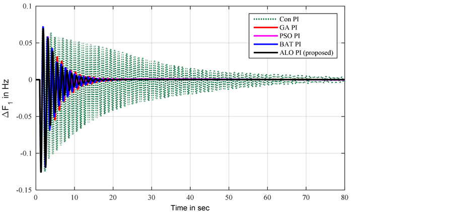
Figure 4. Frequency deviation of area-1 for 10% step increase in load demand in area-1.
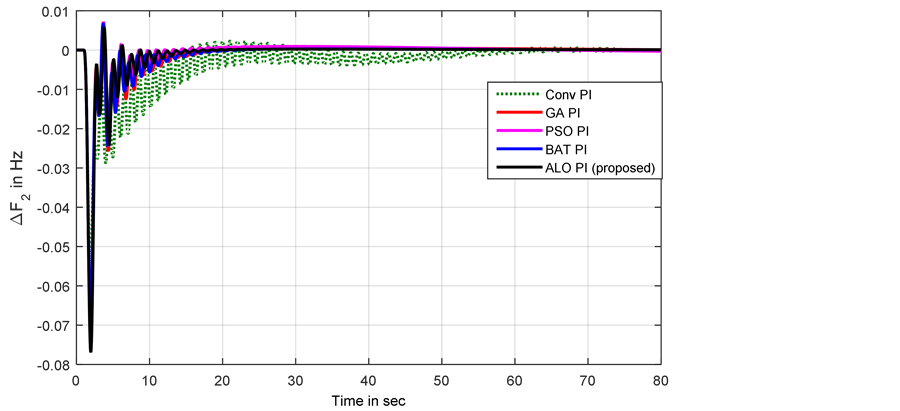
Figure 5. Frequency deviation of area-2 for 10% step increase in load demand in area-1.

Figure 6. Frequency deviation of area-3 for 10% step increase in load demand in area-1.

Figure 7. Tie-line power deviation of area-1 for 10% step increase in load demand in area-1.

Figure 8. Tie-line power deviation of area-2 for 10% step increase in load demand in area-1.

Figure 9. Tie-line power deviation of area-3 for 10% step increase in load demand in area-1.
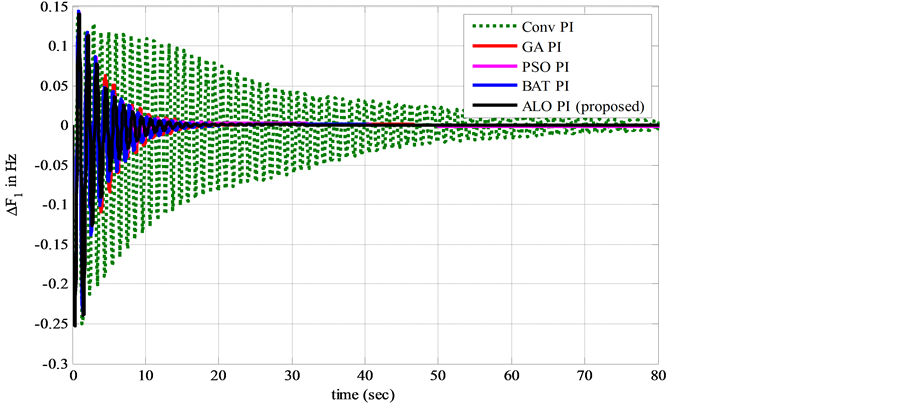
Figure 10. Frequency deviation of area-1 for 20% step increase in load demand in area-1.
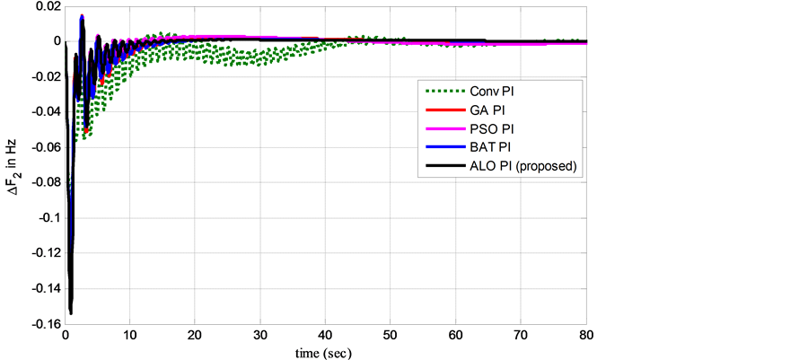
Figure 11. Frequency deviation of area-2 for 20% step increase in load demand in area-1.
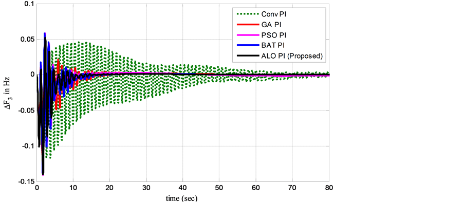
Figure 12. Frequency deviation of area-3 for 20% step increase in load demand in area-1.
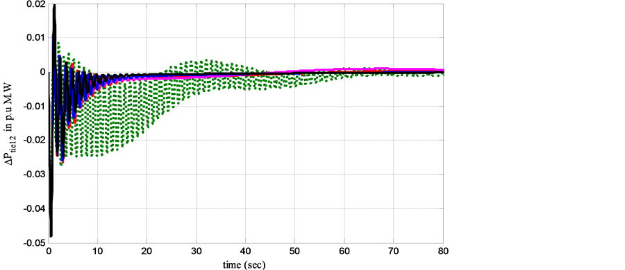
Figure 13. Tie-line power deviation of area-1 for 20% step increase in load demand in area-1.
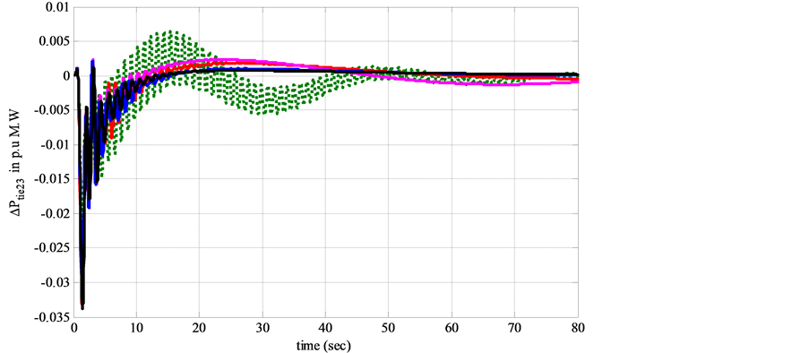
Figure 14. Tie-line power deviation of area-2 for 20% step increase in load demand in area-1.
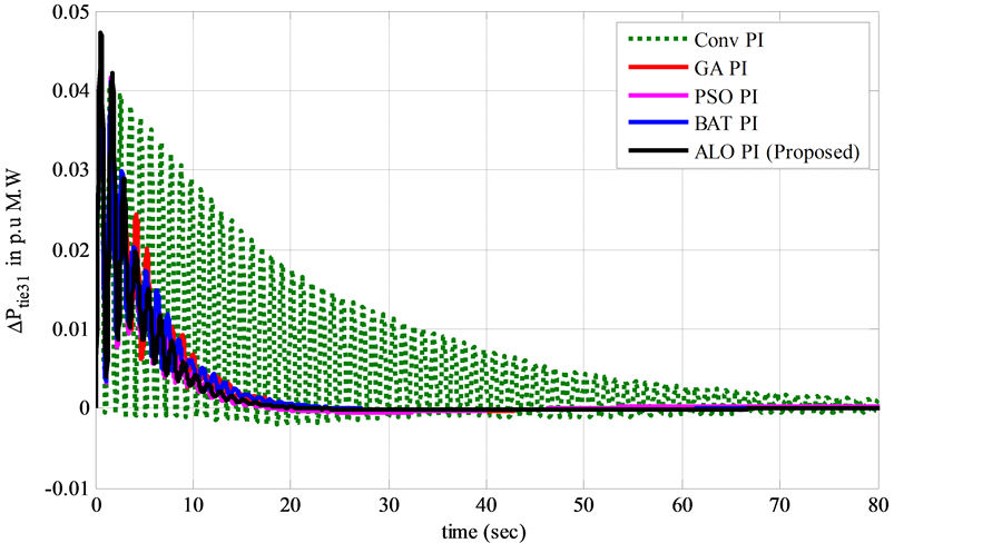
Figure 15. Tie-line power deviation of area-3 for 20% step increase in load demand in area-1.
conditions that, when ITAE is used as an objective function, the system performance with proposed controller is better than that of GA, PSO and BAT based PI controller on ITAE criteria. So, it can be concluded that the performance of proposed ALO is superior to that of GA, PSO, and BAT from fitness function minimization point of view. The response with ALO based PI controller is the best among the other alternatives as best system performance is obtained from desired control specification point of view.
5.2. Case B: Sensitivity Analysis
Sensitivity analysis is carried out to study the robustness the system to wide changes in the operating conditions and system parameters [31] - [33] . The operating load condition and time constants of a speed governor, turbine, tie-line power are varied from their nominal values in the range of +25% to −25%. The change in operating load condition affects the power system parameters KPS and TPS. The power system parameters are calculated for different loading conditions as given in Appendix A. The change in tie-line power is simulated by changing the synchronizing coefficient T12. Figures 16-45 shows the exchanged power between three area under this load exchange. The controller parameters, error performance indices like ITAE, ISE, IAE, frequency and tie line power deviations with various controllers under nominal load and sensitivity load test conditions with time constants of speed governor (Tg), turbine (Tt), tie-line power (T12) and hydraulic governor coefficients (Th1 and Th3) are varied from their nominal values in the range of +25% to −25%. The power system parameters and time constants are calculated for the varied condition and used in the simulation model. In all the cases the controller parameters obtained using the objective function J is considered due to its superior performance. The results obtained are depicted in Table 1 and Table 2. The system performances are within acceptable change when ±25% changes the operating load condition and system parameters from their nominal values. Hence, it can be concluded that the closed loop system is stable when the operating conditions and system parameters vary.
6. Conclusions
ALO algorithm is suggested in this paper to tune the parameters of PI controllers for LFC problem. An integral time absolute error of the ACE for all areas is chosen as the objective function to enhance the system response in terms of the settling time and overshoots. The major contributions of this paper are:
Establishment of the dynamic model for three area power system considering with LFC based Ant Lion Optimizer algorithm to assure the superiority of the PI controller over GA, PSO, BAT and conventional integral controller throughout different disturbances for various signals.
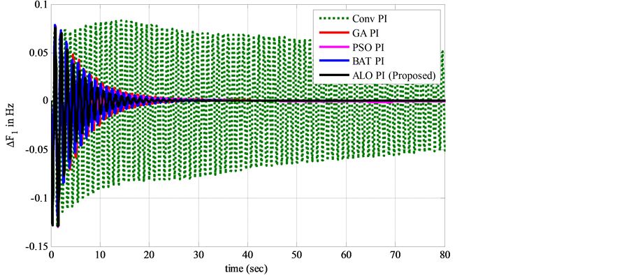
Figure 16. Frequency deviation of area-1 with +25% change in TG.
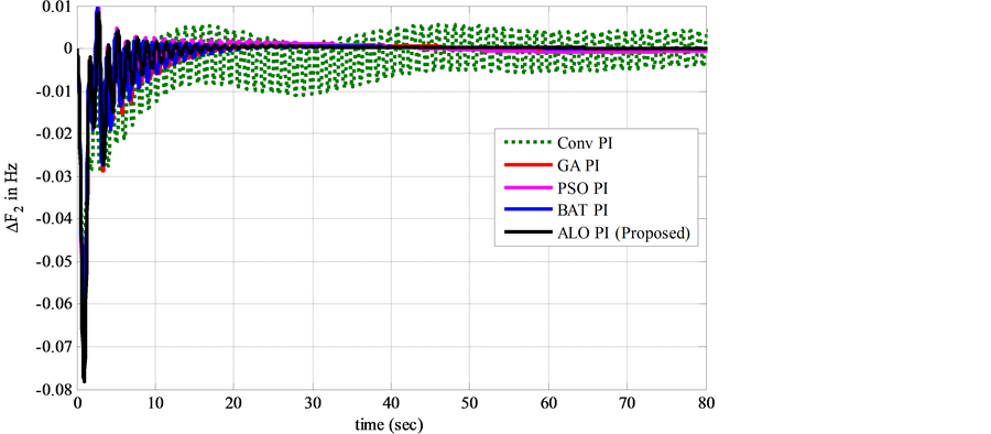
Figure 17. Frequency deviation of area-2 with +25% change in TG.
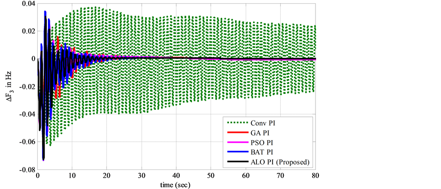
Figure 18. Frequency deviation of area-3 with +25% change in TG.
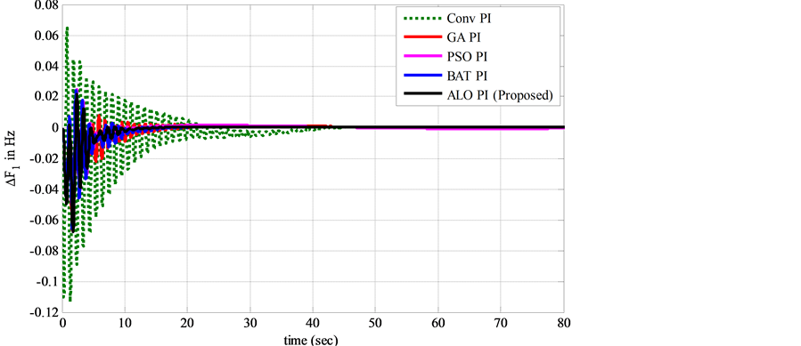
Figure 19. Frequency deviation of area-1 with −25% change in TG.
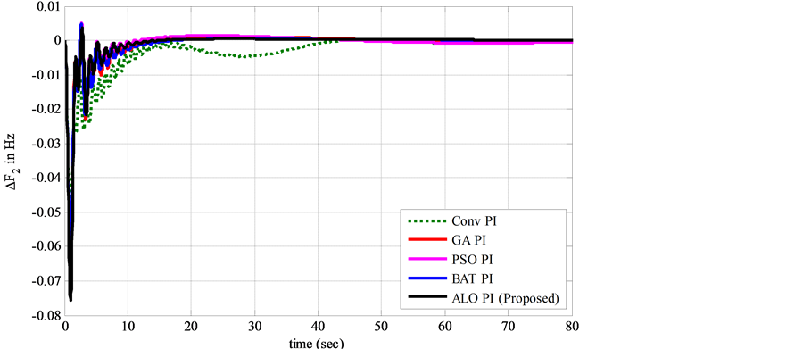
Figure 20. Frequency deviation of area-2 with −25% change in TG.
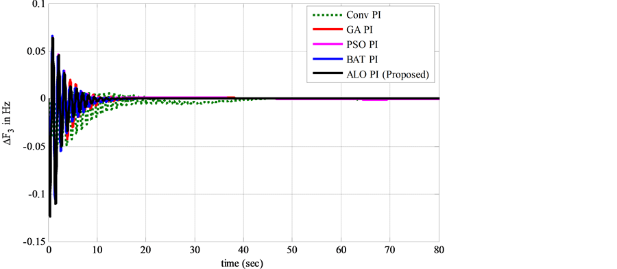
Figure 21. Frequency deviation of area-3 with −25% change in TG.
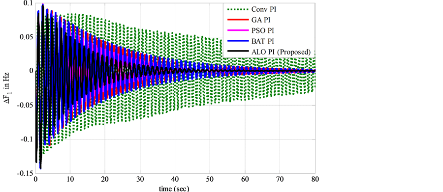
Figure 22. Frequency deviation of area-1 with +25% change in Tt.
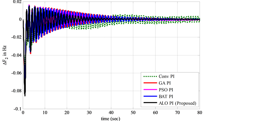
Figure 23. Frequency deviation of area-2 with +25% change in Tt.
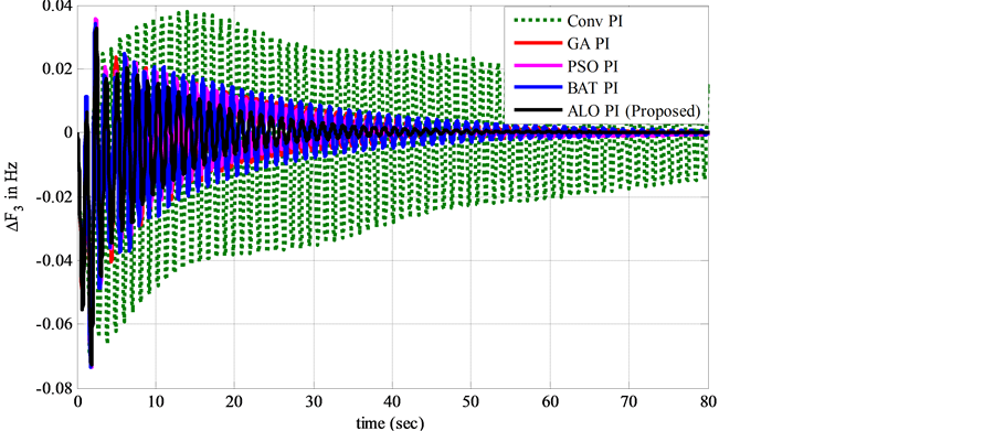
Figure 24. Frequency deviation of area-3 with +25% change in Tt.
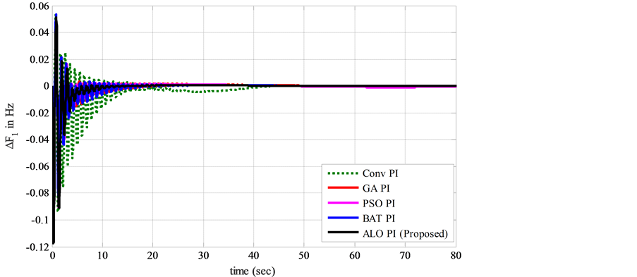
Figure 25. Frequency deviation of area-1 with −25% change in Tt.
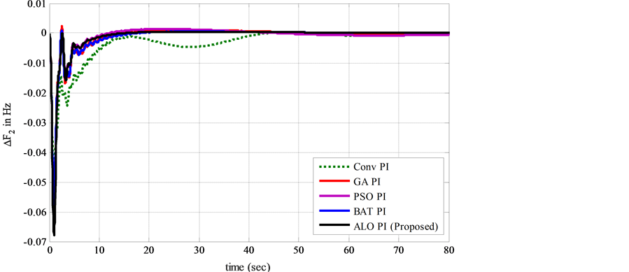
Figure 26. Frequency deviation of area-2 with −25% change in Tt.
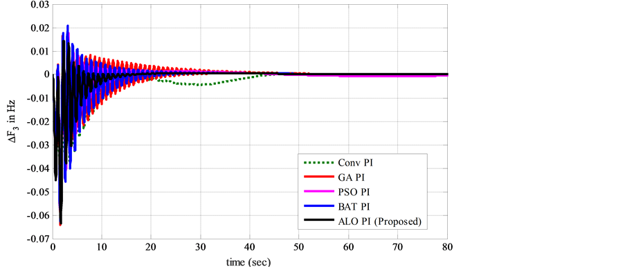
Figure 27. Frequency deviation of area-3 with −25% change in Tt.

Figure 28. Frequency deviation of area-1 with +25% change in Th1.
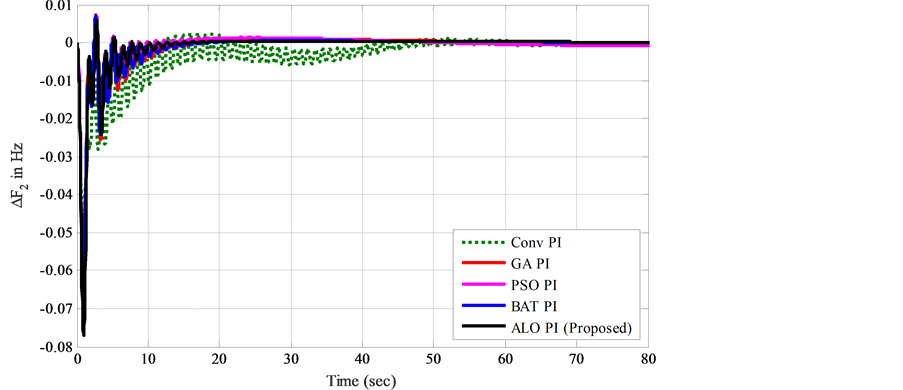
Figure 29. Frequency deviation of area-2 with +25% change in Th1.
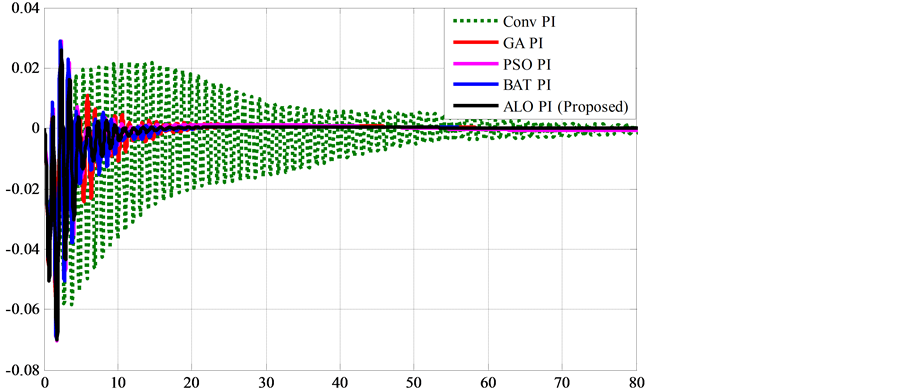
Figure 30. Frequency deviation of area-3 with +25% change in Th1.
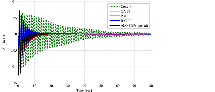
Figure 31. Frequency deviation of area-1 with −25% change in Th1.
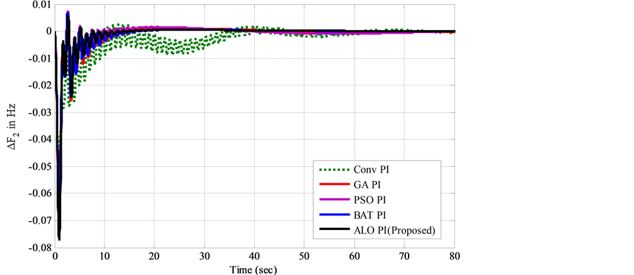
Figure 32. Frequency deviation of area-2 with +25% change in Th1.
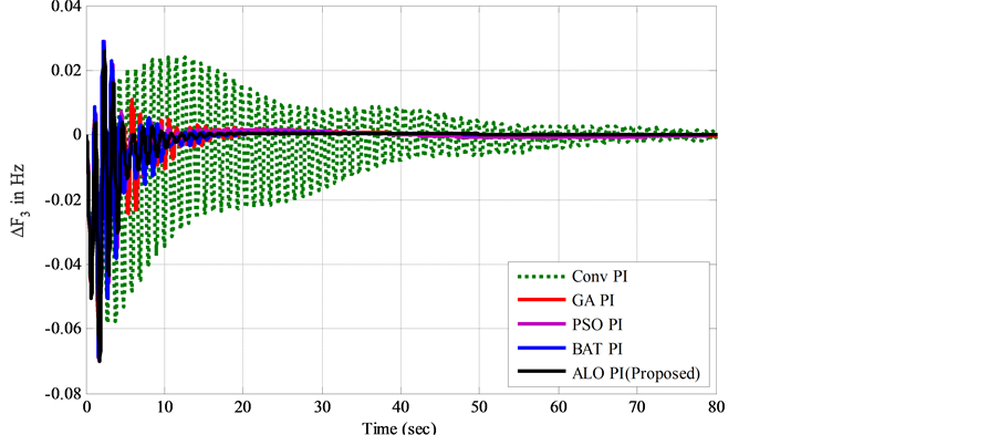
Figure 33. Frequency deviation of area-3 with −25% change in Th1.
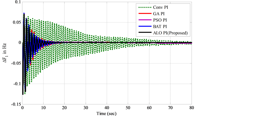
Figure 34. Frequency deviation of area-1 with +25% change in Th3.
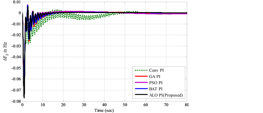
Figure 35. Frequency deviation of area-2 with +25% change in Th3.
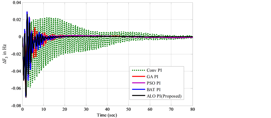
Figure 36. Frequency deviation of area-3 with +25% change in Th3.
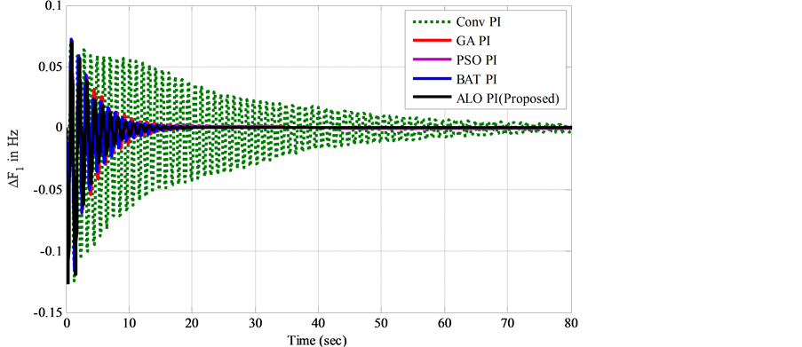
Figure 37. Frequency deviation of area-1 with −25% change in Th3.
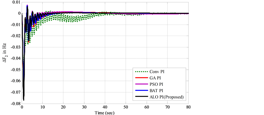
Figure 38. Frequency deviation of area-2 with −25% change in Th3.
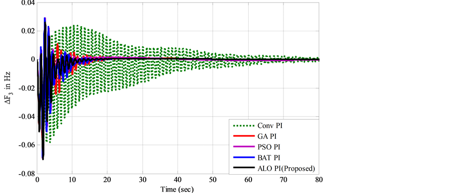
Figure 39. Frequency deviation of area-3 with −25% change in Th3.
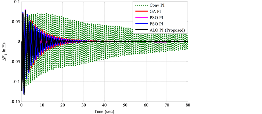
Figure 40. Frequency deviation of area-1 with +25% change in T12.
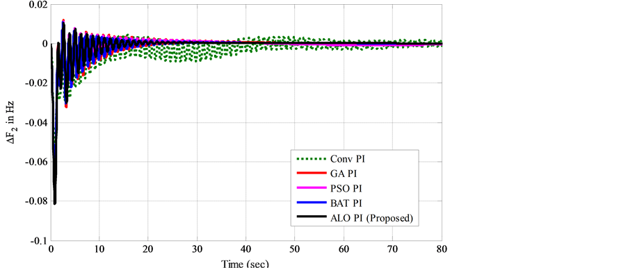
Figure 41. Frequency deviation of area-2 with +25% change in T12.
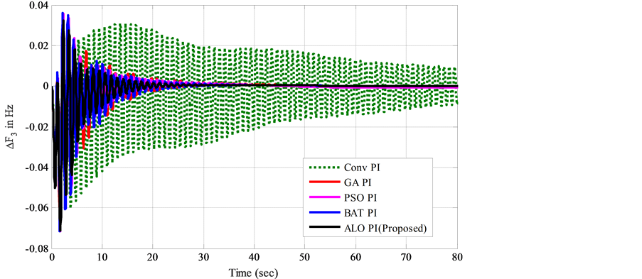
Figure 42. Frequency deviation of area-3 with +25% change in T12.
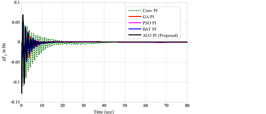
Figure 43. Frequency deviation of area-1 with −25% change in T12.
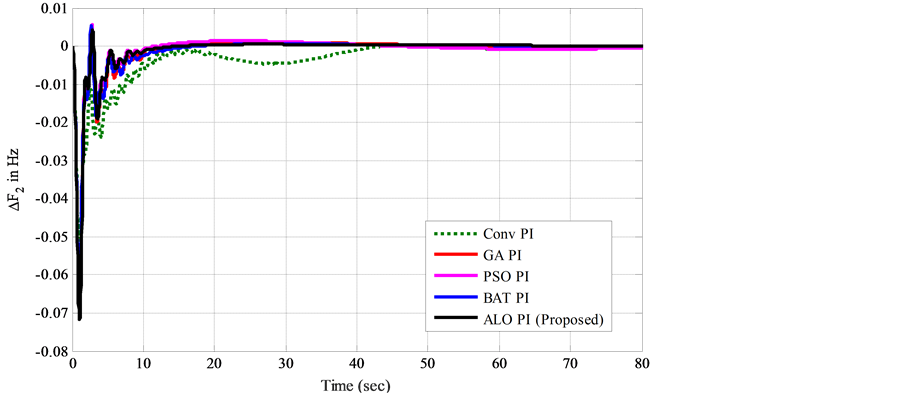
Figure 44. Frequency deviation of area-2 with −25% change in T12.
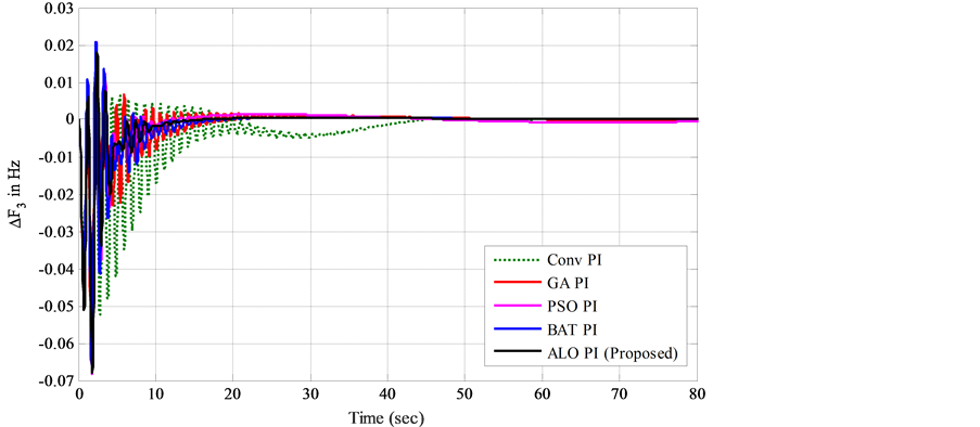
Figure 45. Frequency deviation of area-3 with −25% change in T12.

Table 1. Simulated response of LFC three area interconnected system for case A.
(a) (b)
Table 2. Sensitivity analysis case B.
The robustness of the controller is confirmed through parameter variations. ALO outperforms GA, PSO, BAT in solving LFC problem due to only one parameter required to fine-tune.
On the other hand, GA deals with a population of solutions, thus leading to the disadvantage of requiring a significant number of function evaluations, extensive computational time and gets trapped in local minimum solution. PSO suffers from weak local search ability, and the algorithm may lead to possible entrapment in local minimum solutions. Also, Bat algorithm exploitation stage too quickly by varying loudness and pulse rates quickly, it can result in stagnation after some initial stage.
The capability of the developed controllers to compensate the communication time delay and preserve its satisfactory performance is demonstrated.
The effectiveness of the controller regarding various indices and settling time is proved.
Acknowledgements
Nominal parameters of the three area system investigated are [12] : PR = 2000 MW (rating), PL = 1000 MW (nominal loading); f = 60 Hz, B1=B2 = 0.425 p.u. MW/Hz; R1= R2 = 2.4 Hz/p.u.; Tg1 = 0.08 s; Tt1 = 0.3 s; KPS1 = KPS2 = KPS3 =120 Hz/p.u. MW; TPS1 = TPS2 =TPS3 = 20 s; T12 = T23 = T31 = 0.545 pu; Th1 = 48.7s; Th2 = 0.513s; Th3 = 10s; Thw = 1.0s.
Cite this paper
R. Satheeshkumar,R. Shivakumar, (2016) Ant Lion Optimization Approach for Load Frequency Control of Multi-Area Interconnected Power Systems. Circuits and Systems,07,2357-2383. doi: 10.4236/cs.2016.79206
References
- 1. Shayeghi, H., Shayanfar, H.A. and Jalili, A. (2009) Load Frequency Control Strategies: A State-of-the-Art Survey for the Researcher. Energy Conversion and Management, 50, 344-353.
http://dx.doi.org/10.1016/j.enconman.2008.09.014 - 2. Kundur, P. (2009) Power System Stability and Control. TMH.
- 3. Elgerd, O.I. (1983) Electric Energy Systems Theory. An Introduction. Tata McGraw-Hill, New Delhi.
- 4. Ibraheem, Kumar, P. and Kothari, D.P. (2005) Recent Philosophies of Automatic Generation Control Strategies in Power Systems. IEEE Transactions on Power Systems, 20, 346-357.
- 5. Mohamed, T.H., Bevranib, H., Hassand, A.A. and Hiyamac, T. (2011) Decentralized Model Predictive Based Load Frequency Control in an Interconnected Power System. Energy Conversion and Management, 52, 1208-1214.
http://dx.doi.org/10.1016/j.enconman.2010.09.016 - 6. Daneshfar, F. and Bevrani, H. (2010) Load-Frequency Control: A GA-Based Multi-Agent Reinforcement Learning. IET Generation, Transmission & Distribution, 4, 13-26.
http://dx.doi.org/10.1049/iet-gtd.2009.0168 - 7. Saikia, L.C., Nanda, J. and Mishra, S. (2011) Performance Comparison of Several Classical Controllers in AGC for Multi-Area Interconnected Thermal System. International Journal of Electrical Power & Energy Systems, 33, 394-401.
http://dx.doi.org/10.1016/j.ijepes.2010.08.036 - 8. Nanda, J., Mishra, S. and Saikia, L.C. (2009) Maiden Application of Bacterial Foraging Based Optimization Technique in Multi-Area Automatic Generation Control. IEEE Transactions on Power Systems, 24, 602-609.
http://dx.doi.org/10.1109/TPWRS.2009.2016588 - 9. Ali, E.S. and Abd-Elazim, S.M. (2011) Bacteria Foraging Optimization Algorithm Based Load Frequency Controller for Interconnected Power System. International Journal of Electrical Power & Energy Systems, 33, 633-638.
http://dx.doi.org/10.1016/j.ijepes.2010.12.022 - 10. Shabani, H., Vahidi, B. and Ebrahimpour, M. (2012) Robust PID Controller Based on Imperialist Competitive Algorithm for Load-Frequency Control of Power Systems. ISA Transactions, 52, 88-95.
http://dx.doi.org/10.1016/j.isatra.2012.09.008 - 11. Rout, U.K., Sahu, R.K. and Panda, S. (2013) Design and Analysis of Differential Evolution Algorithm Based Automatic Generation Control for Interconnected Power System. Ain Shams Engineering Journal, 4, 409-421.
http://dx.doi.org/10.1016/j.asej.2012.10.010 - 12. Panda, S., Mohanty, B. and Hota, P.K. (2013) Hybrid BFOA-PSO Algorithm for Automatic Generation Control of Linear and Non-Linear Interconnected Power Systems. Applied Soft Computing, 13, 4718-4730.
http://dx.doi.org/10.1016/j.asoc.2013.07.021 - 13. Rakhshani, E. (2012) Intelligent Linear-Quadratic Optimal Output Feedback Regulator for a Deregulated Automatic Generation Control System. Electric Power Components and Systems, 40, 513-533.
http://dx.doi.org/10.1080/15325008.2011.647239 - 14. Ibraheem, Kumar, P., Hasan, N. and Nizamuddin (2012) Suboptimal Automatic Generation Control of Interconnected Power System Using Output Vector Feedback Control Strategy. Electric Power Components and Systems, 40, 977-994.
http://dx.doi.org/10.1080/15325008.2012.675802 - 15. Huang, C.X., Zhang, K.F.,Dai, X.Z. and Zang, Q. (2013) Robust Load Frequency Controller Design Based on a New Strict Model. Electric Power Components and Systems, 41, 1075-1099.
http://dx.doi.org/10.1080/15325008.2013.809824 - 16. Jazaeri, M. and Chitsaz, H. (2011) A New Efficient Scheme for Frequency Control in an Isolated Power System with a Wind Generator. Electric Power Components and Systems, 40, 21-40.
http://dx.doi.org/10.1080/15325008.2011.621921 - 17. Yang, X.S. (2008) Nature-inspired Metaheuristic Algorithms. Luniver Press, UK.
- 18. Yang, X.S. (2009) Firefly Algorithms for Multi-Modal Optimization. In: Watanabe, O. and Zeugmann, T., Eds., Stochastic Algorithms: Foundations and Applications, Springer, Berlin, 169-178.
http://dx.doi.org/10.1007/978-3-642-04944-6_14 - 19. Yang, X.S. (2010) Firefly Algorithm, Stochastic Test Functions, and Design Optimization. International Journal of Bio-Inspired Computation, 2, 78-84.
http://dx.doi.org/10.1504/IJBIC.2010.032124 - 20. Yang, X.-S., Hosseini, S.S.S. and Gandomi, A.H. (2012) Firefly Algorithm for Solving Non-Convex Economic Dispatch Problems with Valve Loading Effect. Applied Soft Computing, 12, 1180-1186.
http://dx.doi.org/10.1016/j.asoc.2011.09.017 - 21. Saikia, L.C. and Sahu, S.K. (2013) Automatic Generation Control of a Combined Cycle Gas Turbine Plant with Classical Controllers Using Firefly Algorithm. International Journal of Electrical Power & Energy Systems, 53, 27-33.
http://dx.doi.org/10.1016/j.ijepes.2013.04.007 - 22. Chandrasekaran, K., Simon, S.P. and Padhy, N.P. (2013) Binary Real Coded Firefly Algorithm for Solving Unit Commitment Problem. Information Sciences, 249, 67-84.
http://dx.doi.org/10.1016/j.ins.2013.06.022 - 23. Senthilnath, J., Omkar, S.N. and Mani, V. (2011) Clustering Using Firefly Algorithm: Performance Study. Swarm and Evolutionary Computation, 1, 164-171.
http://dx.doi.org/10.1016/j.swevo.2011.06.003 - 24. Abdel-Magid, Y.L. and Dawoud, M.M. (1995) Genetic Algorithms Applications in Load Frequency Control. 1st International Conference on Genetic Algorithms in Engineering Systems: Innovations and Applications, Sheffield, 12-14 September 1995, 207-213.
- 25. Jeddi, S.A., Abbasi, S.H. and Shabaninia, F. (2012) Load Frequency Control of Two Area Interconnected Power System (Diesel Generator and Solar PV) with PI and FGSPI Controller. The 16th CSI International Symposium on Artificial Intelligence and Signal Processing (AISP 2012), Shiraz, 2-3 May 2012, 526-531.
- 26. Prakash, S. and Sinha, S.K. (2014) Simulation-Based Neuro-Fuzzy Hybrid Intelligent PI Controls Approach in Four-Area Load Frequency Control of Interconnected Power System. Applied Soft Computing, 23, 152-164.
http://dx.doi.org/10.1016/j.asoc.2014.05.020 - 27. Panda, S., Mohanty, B. and Hotab, P.K. (2013) Hybrid BFOA-PSO Algorithm for Automatic Generation Control of Linear and Nonlinear Interconnected Power Systems. Applied Soft Computing, 13, 4718-4730.
http://dx.doi.org/10.1016/j.asoc.2013.07.021 - 28. Ali, E.S. and Abd-Elazim, S.M. (2011) Bacteria Foraging Optimization Algorithm Based Load Frequency Controller for the Interconnected Power System. International Journal of Electrical Power & Energy Systems, 33, 633-638.
http://dx.doi.org/10.1016/j.ijepes.2010.12.022 - 29. Abdelaziz, A.Y. and Ali, E.S. (2015) Cuckoo Search Algorithm Based Load Frequency Controller Design for the Nonlinear Interconnected Power System. International Journal of Electrical Power & Energy Systems, 73, 632-643.
http://dx.doi.org/10.1016/j.ijepes.2015.05.050 - 30. Mirjalili, S. (2015) The Ant Lion Optimizer. Advances in Engineering Software, 83, 80-98.
http://dx.doi.org/10.1016/j.advengsoft.2015.01.010 - 31. Gozde, H., Taplamacioglu, M.C. and Kocaarslan, I. (2012) Comparative Performance Analysis of Artificial Bee Colony Algorithm in Automatic Generation Control for Interconnected Reheat Thermal Power System. International Journal of Electrical Power & Energy Systems, 42, 167-178.
http://dx.doi.org/10.1016/j.ijepes.2012.03.039 - 32. Parmar, K.P.S., Majhi, S. and Kothari, D.P. (2012) Load Frequency Control of a Realistic Power System with Multi-Source Power Generation. International Journal of Electrical Power & Energy Systems, 42, 426-433.
http://dx.doi.org/10.1016/j.ijepes.2012.04.040 - 33. Panda, S. and Yegireddy, N.K. (2013) Automatic Generation Control of Multi-Area Power System Using Multi-Objective Non-Dominated Sorting Genetic Algorithm-II. International Journal of Electrical Power & Energy Systems, 53, 54-63.
http://dx.doi.org/10.1016/j.ijepes.2013.04.003