ABSTRACT

In this work some characteristics and applications for quantum information is revealed. The various dynamical equations of quantum information density have been investigated, transmission characteristics of the dynamical mutual information have been studied, and the decoherence-free controlling procedure has been considered, which exposes that quantum information is holographic through the similarity structure of subdynamic kinetic equations for quantum information density.

1. Introduction

Since quantum information theory has made great progresses, it has expanded to treat the intact transmission and processing of quantum states, entanglement of states, offers potentially great advantages over classical information processing, both for efficient algorithms [1,2] and for secure communication [3,4]. Many different implementations for quantum information have been proposed based on principles of quantum computation, quantum cypotography or quantum teleportation, such as Deutsch’s work [5], Shor algorithm for factoring large numbers [6] and the Grover algorithm for search in an unstructured database [7]. However, until recently it has not been clear what is fundamental dynamical equation directly related to quantum information, except this one, in this work we studied three interesting problems raised: 1) Is the transmission of the quantum information related to the dyanmical process in the mutual information? 2) Is quantum information holographic through the similarity structure of subdynamic kinetic equation? 3) How does one control quantum decoherence in the canonical ensemble system?

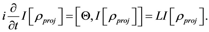
2. Dynamical Equations for Quantum Information Density

First question answer is: the Liouville equation, the Schwinger-Tomonaga equation and the Einstein equation still hold for quantum information density (QID). In this sense the universe is unified to quantum information, and is driven by the Hamiltonian (energy). In fact, as many physical researchers well know, from Schrödinger equation, through derivative to both side of density operator, one can obtain a Liouville equation as

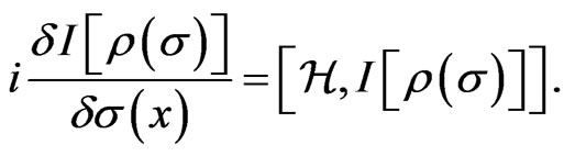
Then, by using the Liouville equation one can find that the Liouville equation is true for, continuing this procedure until, for any integer n, one can see that the Liouville equation is still true, finally, one can concludes that the Liouville equation still holds for any analytic functional of,

(1)

The physical meaning of the above equation can be explained as “a general dynamical relation of information and energy”, here, Hamiltonian H corresponding to the energy, and corresponding to a general quantum information, especially, is a quantum information density (QID). In this way we define that is to correspond upon the quantum information means 1) can be expanded as the power series of, which may be defined as a generalized (or advanced) quantum information density, 2) is quantum information density, 3) can be considered as a minimum unit of the quantum information density. Moreover, in the classical system, the Liouville equation for the information density can also be established by

(2)

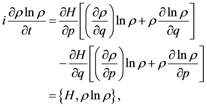
where defined as a Poisson Bracket. Because QID is just the negative entropy density, this physical meaning of QID allow us to consider logically introduce a micro-representation of the second law of thermodynamics by

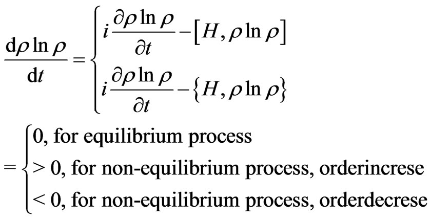(3)

which gives naturally a general Liouville equation for a non-equilibrium process constructed by

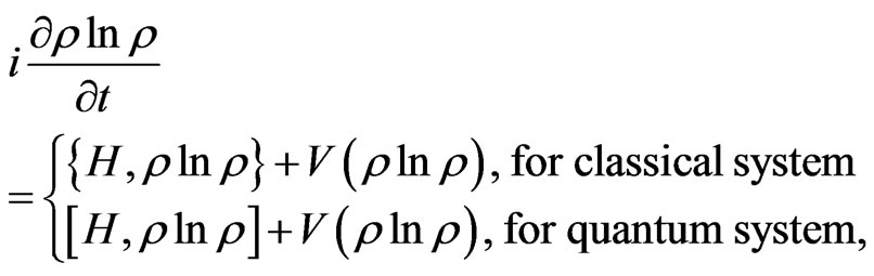(4)

where is assumed to be introduced by the difference of QID within the systems or between the system and environment. More generally, this difference is supposed to be introduced by a potential of information density, which drives the system evolves along the direction described by the second law of thermodyanmics.

The above fundamental Equation (1) can be expanded to the general relativity system. Indeed, the SchwingerTomonaga equation for the density operator presented by Schwinger and Tomomaga [8-12] is

(5)

where denotes the Hamiltonian density, is three-dimensional spacelike hypersurface defined to be a three-dimensional manifold in Minkowski space. Each point defined as for the space-time coordinates. Formally, the functional derivative is defined as

(6)

where the volume of the four-dimensional space-time region enclosed by and is denoted by. Hence, the solution of the Schwinger-Tomonaga equation can be written by

(7)

where

(8)

denotes the chronological time-ordering operator. The density operator then becomes a functional on the set of spacelike hypersurfaces. For deriving the Schwinger-Tomonaga equation for functional of, we start from the Schwinger-Tomonaga equation and have:

(9)

for any integer. Considering for any analytic functional of, can be expanded as a power series on, a Schwinger-Tomonaga equation for general functional of thus can be obtained by

(10)

The above established Schwinger-Tomonaga equation for QID allows one to study QID dynamics in curved space-time. In fact again, the above Schwinger-Tomonaga equation can also be extended to the curved spacetime by introducing the quantum bundles and the covariant derivative to replace the ordinary derivative, thus, in the general relativistic domain the state vector or the functional of density operator must be regarded as a functional of the set of spacelike hypersurfaces in curved space-time manifold [10,13]. Then, let the Hamiltonian density of gravitation field and matter be described by 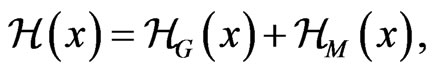where represents the Hamiltonian density of gravity field whose Lagrangian density is given by Einstein-Hilbert action, , and represents the Hamiltonian density of the matter. Thus, in terms of Equation (10) a general functional of density operator (or) defined as quantum information field density satisfies the Schwinger-Tomonaga equation. Taking variation of with respect to reverse metric, which gives an interesting equation:

(11)

where

We neglect second order variation, which results in

(12)

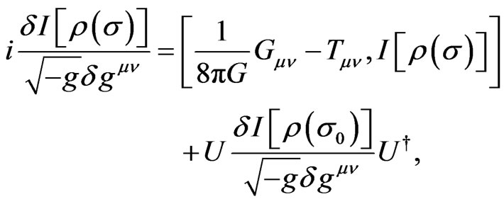
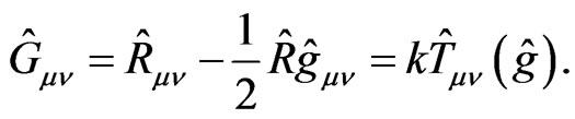
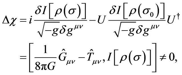
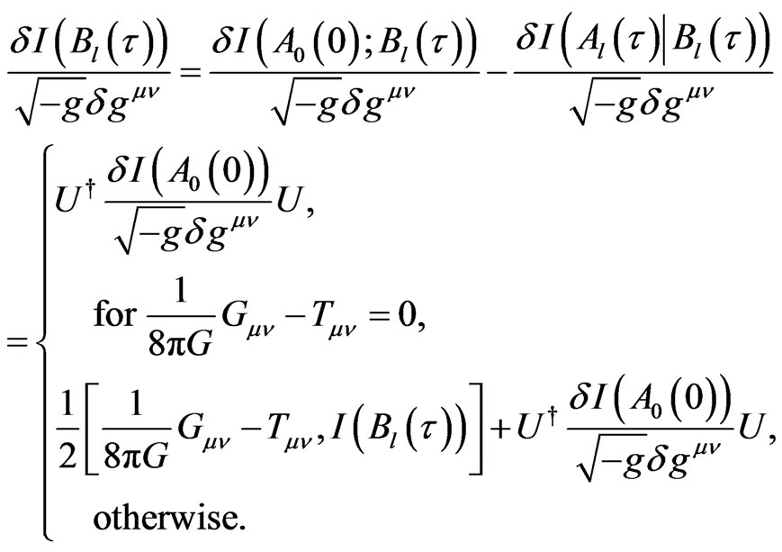
The established Equation (11) may be a quite interesting equation which is related to the Einstein equation, general functional of density operator (including density operator or quantum information density) and the Schwinger-Tomonaga equation. In fact, based on the theory of quantum gravity, such as the Loop quantum gravity [14] or formalism of geometro-stochastic approach [13], the Einstein equation can be formally quantized as the quantum Einstein equation:

This gives

Hence one has the evolution equation for 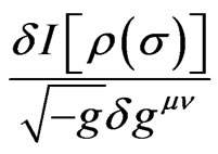from Equation (11), which shows an interesting evolution symmetric property for (general) QID in the timespace:

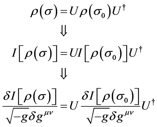(13)

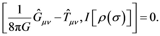
in which the Schwinger-Tomonaga equation (including Liouville equation, Schrödinger equation) and Einstein equation (including quantum Einstein equation) are implied. This shows that the fundamental dynamical processes are related to QID. Moreover, since in quantum fluctuations, virtual pairs of positive and negative electrons, in effect, are continually being created and annihilated, and likewise pairs of mu mesons, pairs of baryons, and pairs of other particles, all these fluctuations should coexist with the quantum fluctuations in the geometry and topology of space. Then it is possible that the quantum Einstein equation is induced an additional disturbance (as a sort of potential of information density) as

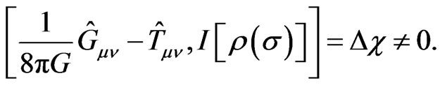(14)

One interesting evidence is the vacuum, i.e. if the state with respect to which the expectation value is taken is the vacuum state with respect to so that

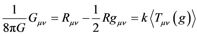(15)

then the right side of the above equation is generally non-vanishing because of the vacuum fluctuations. This possible large fluctuation of metric operator can not be ignored in extreme astrophysical or cosmological situations, such as near a black hole or big bang singularity [14]. If it is so the Equation (11) can describe the QID fluctuation as

(16)

where may be an imaginary value, which means that the QID fluctuation may cause derivation of the Einstein equation in quantum levels.

3. Dynamical Mutual Information

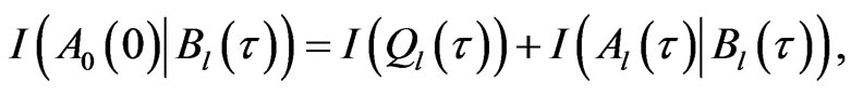
The second answer is: the transmission of quantum information along with the dynamical evolution. The both processes can be closely relevant. Indeed, for measuring, it may be important to calculate the mutual information in the system. Generally, starting from the definition of the mutual information density we have [15]:

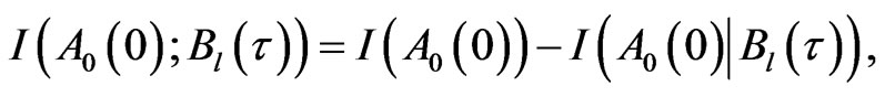(17)

(18)

where is an input ensemble encoded state at time with special coordinate which is the channel length, is an output ensemble encoded state at time with the coordinate, is accumulated lost information density in the channel. When the transmitting time of QID or symbols through channel is long enough with noise in the transmission process, the receiver receive the amount of information contained in the at the time and the output terminal with respect to the which transmitted by transmitter at the time and the input terminal. This is dynamical mutual information. The motivation to propose this formalism is to consider that the quantum channel has long size and noise in transmission process which is different from the usual “point” model of the channel (or zero transmitting time model) [15]. Thus, the is given by

(19)

This allows the dynamical mutual QID is obtained by

(20)

This shows that the initial quantum signal (QID) also transform l coordinate from 0 during time in the quantum channel. We emphasize again that the channel possessing dimensional size l and transmission time is different from the traditional quantum (or classical) channel which only represents certain mathematical mapping without physical size and passing time. The above formula shows that the evolution of QID influence the dynamical mutual QID by which can be described by the kinetic equation of QID. Thus, one gets

(21)

where is output, and

(22)

For example, considering a harmonic oscillator interacting with a quantum gravitational radiation field g, the relevant Hamiltonian is described by

with

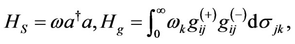
and

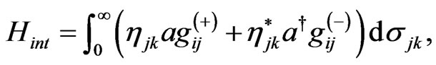
where is the creation (annihilation) operator for the oscillator in a Fock fibre, is the creation (annihilation) operator of the k continuum field mode (or graviton) within a graviton fibres, is the Lamour frequency of spin k due to the Zeeman interaction, and denotes the coupling between the oscillator and field mode [13]. Generally, from the Schwinger-Tomonaga equation for a general functional of, , one can get the Liouville equation for; based on this, a master equation for the functional of the reduced density operator can be obtained [16], which results in a quantum Fokker-Planck equation for in the coherent representation (QFPE). This QFPE may describe transmission of the information density signals (encoded in harmonic oscillator) along a quantum Gaussian channel by extending the concept of classical Gaussian channel for information. Concretely, let us consider a harmonic oscillator as ebit encoded quantum information on their coherent states. This oscillator consisting of photons is like the Brownian particle transmission in an information channel described by QFPE, i.e. the channel can be described by evolution operator induced by QFPE acting on initial input QID. When the oscillator consisting of photons are transmitted from the input system, the oscillators consisting of photons from the noise system (environment) add to the signal, then photons are lost to the loss system through the channel, and photons are detected in the output system, with [17]. Furthermore, if the spectral decomposition of the density operator for the mixed states of photons is given by then its QID transmission in the channel remains the same quantum entanglement (parallelism) described by the spectral decomposition of the functional: , where defined as a quantum information. This makes the quantum Gaussian channel to have an (parallelism) advantage over classical Gaussian channel.

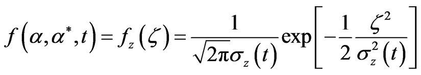
The solution of QFPE is given by [18]. By substituting into the Gaussian ansatz, one obtains the solution as

(23)

with, where and represent the mean power of input signal and noise, respectively, they are assumed to correspond to the Gaussian distributed random variables [19]. Then the solution gives a formulation of the Bayesian estimation, which derives a condition information, then using Gaussian integral properties one finally obtain a quantum dynamical mutual information formula [15,16] for the quantum Gaussian channel in the coherent state representation,

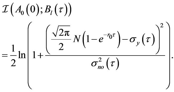(24)

where and have the same definitions as previously explanations. Hence Equation (24) can be used for measuring the variation of QID,.

For instance, a condition for the QID fluctuation in the Gaussian channel is given by

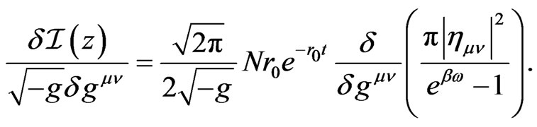(25)

This gives a condition for the QID fluctuation

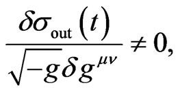(26)

when is a function of metric, which is coincidence with the definition of in the interaction Hamiltonian, i.e. is the coupling between the oscillator and field mode. This shows that the fluctuation of QID with the metric in curved time-space may exist and be related to the (quantum) Einstein equation. A significant condition for this QID fluctuation is that the coupling number of the system with the gravitation is a function of the metric on curved space-time manifold.

4. Quantum Information Holography through SKE

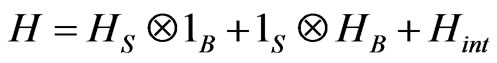
The third question answer is that QID is holographic through the similarity of subdynamic kinetic equation (SKE). For making this point, we try to introduce a subdynamic formalism [20-22] and followed by some recent works [23,24]. In fact, let a quantum system S be coupled to a thermal reservoir B, H_S, H_B, and denote the Hamiltonian of the system S, the Hamiltonian of the thermal reservoir B, and the interaction between S and B, respectively. The total Hamiltonian H of the system plus the reservoir can be expressed as . Then in terms of the corresponding quantum Schrödinger equation and Liouville equation, one can introduce a basis, , where j is an index denoting S system and k is an index denoting thermal reservoir B. Usually the basis, is chosen as complete set of eigenvectors of the free Hamiltonian, , here for generally, the can be chosen as any suitable complete basis in the Hilbert space spanned by the eigenvectors of. 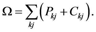Hence the orthonormal projector (or) can be introduced by the basis, with, so that

(27)

where is a diagonal part of the Hamiltonian expanded by the basis and is an offdiagonal part of the Hamiltonian expanded by the basis. Then the total Hamiltonian H can be expressed by a projected matrix, which allows one to introduce a creation (destruction) correlation operator (as a type of resolvent) by

(28)

(29)

This shows that the is an eigenvector of the , and is an joint eigenvalue of , which permits one to get the eigenvector of H as with the same eigenvalue. Using above equations, by introducing as an eigen-projector of H, one can construct a Schrödinger type of SKE for each projected state as

(30)

with

(31)

where and are defined as

(32)

and or is a solution of the original Schrödinger equation, which may be in the Rigged Hilbert space, , , is a dense subspace of the Hilbert space, and is a dual space of.

Furthermore, by replacing, and using the above SKE, a Liouvillian type of SKE can also be derived by

(33)

The construction of the Schrödinger (Liouvillian) type of SKE in subspace can be intertwined to the original Schrödinger (Liouville) equation with the same spectral structure between operator and Hamiltonian (Liouvillian) [20,23]. For instance, using the relation (30) one has the spectral representation of H related to as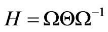, where, and

(34)

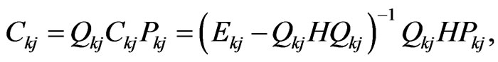
The creation operator,

(35)

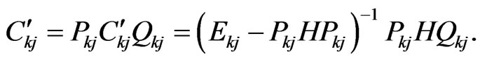
creates the -part of from the -part. While

(36)

is called intermediate (collision) operator [20]. This may be a kind of information holography between the original Schrödinger (Liouvillian) equation and SKE, which means for every basic dynamical equation one can construct its SKE by projecting procedure, and both equations intertwine with each other by the similarity transformation. This may be described as following similarity structure:

(37)

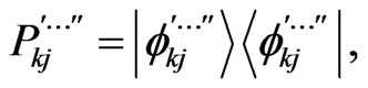
where the first index means 1-order of the SKE, and the second index means 2-order of the SKE, until that n-order, ···. The higher order of represents the “vacuum” part of the “dynamic” part of the lower order of density operator, which describes the essence of information contained in the density in its own subspace [25]. This is phyical meaning of holography here. Marvelously this holographic formalism can be generally used to solve the eigenvalues problem for the Schrödinger (Liouville) equation generally as below: indeed, if is an eigen-projector of, then from the SKE one gets the eigenvector of H is given by

(38)

and the eigenvalue of H is given by

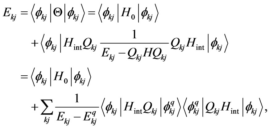(39)

where defining, and suppose the spectral decomposition of is

(40)

and the eigenvalue can be gotten by using the SKE again,

(41)

Continuing this procedure until finally one has only containing 1 projector

(42)

then one gets the eigen-vector as

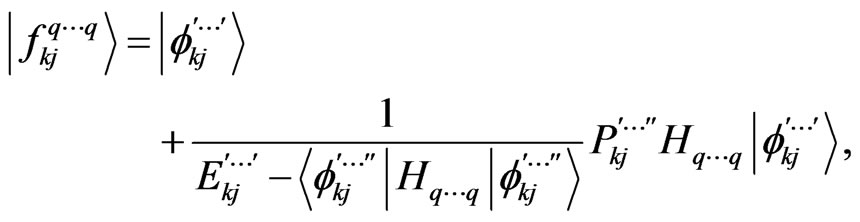(43)

and the eigenvalus as

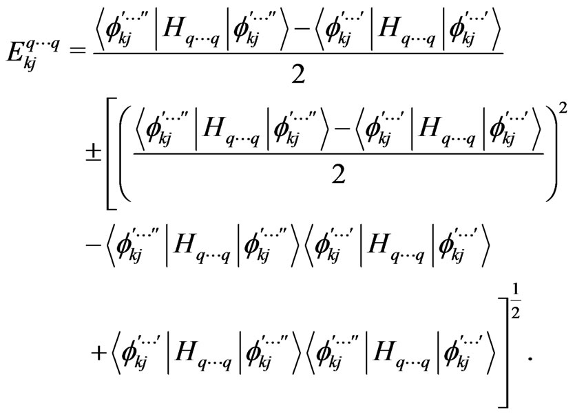(44)

Replacing back the final result to the previous currency formalism, eventually one can obtain the eigenvector (eigenvalue) of H.

For example, let us consider a Heisenberg model related to three spins interaction with each others. Its Hamiltonian is expressed by

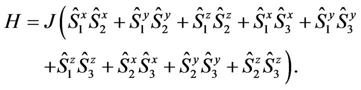(45)

Choosing a basis as

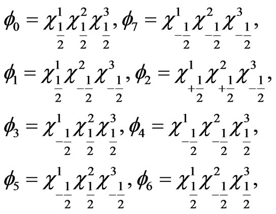(46)

the diagnal matrix elements of H can be given by

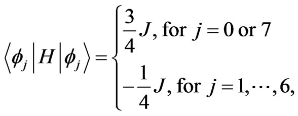(47)

and the off-diagnal matrix elements of H can be given by

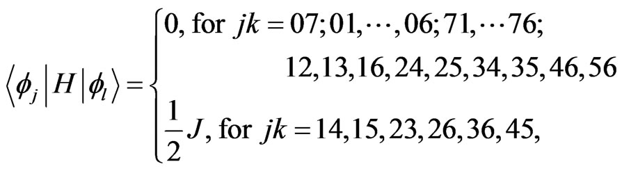(48)

where notice the index j or k as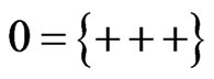, , , , , , ,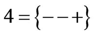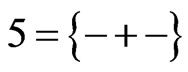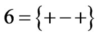. The eigenvalues and eigenvectors can be calculated by the above presented formalism. Firstly it is obvious that 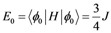, and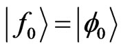. Furthermore, the eigenvalues and eigenvectors of the 6-order of projection hamiltonian are given, such as

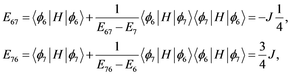(49)

and

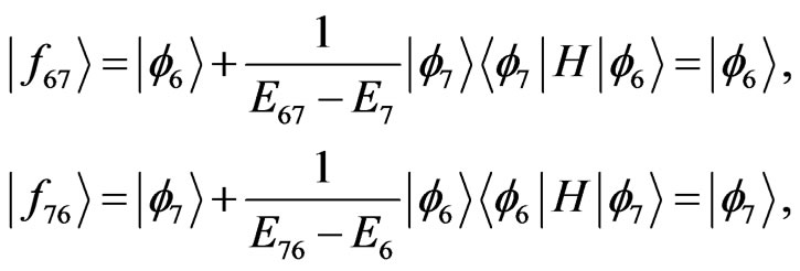(50)

···, continuing untill one gets the eigenvalues and eigenvectors of the 1-order of projection hamiltonian, such as

(51)

and

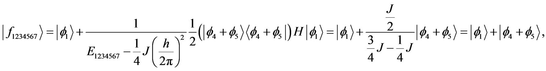(52)

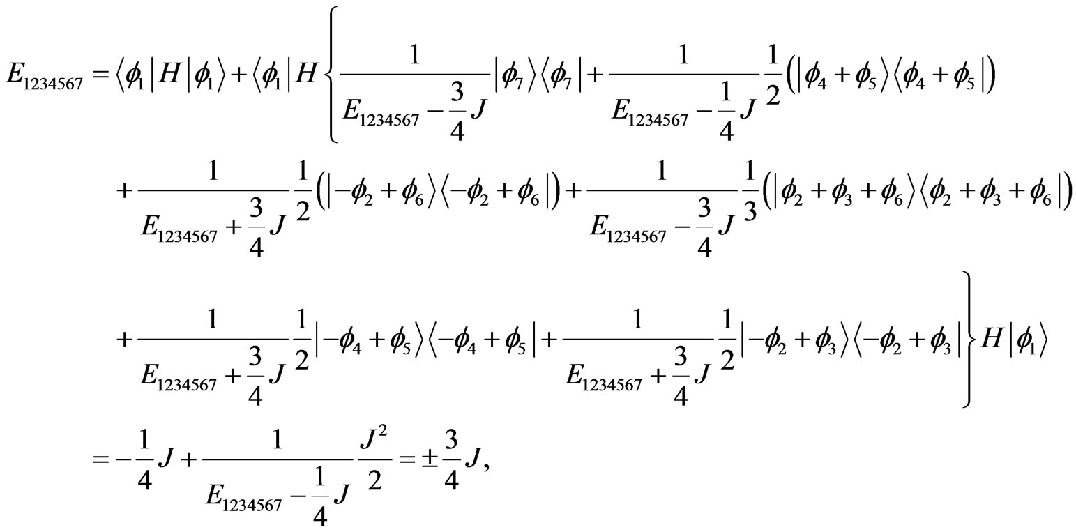
and so on, finally author obtains the eigenvector and eigenvalues of the Hamiltonian expressed by

(53)

(54)

This example shows that the above procedure to gain the eigenvalues and eigenvectors is corret.

5. The Decoherence-Free Control

The fourth problem answer is that the decoherence can be controlled by using a non-eqilibrium statistical ensembles formalism based on the SKE. Indeed again, the physical meaning of is that it represents the “vacuum” part of the “dynamic” part of the original density operator, which describes the essence of (irreversible) evolution of the density in its own subspace [25]. The second order approximation of with respect to corresponds to the Master equation [22] derived by using the Zwanzig projection technique, and the Boltzmann, Pauli, and Fokker-Planck equations of kinetic theory and Brownian motion can also be derived by using some approximation of [25]. Author would like to clarify that although using the Zwanzig projection technique, the (differential integral) Master equation for the relevant part of the density operator in Liouvillian space can also be derived [26,27], but the Schrödinger type of differential equation as SKE in subspace can not be derived by the Zwanzig projection technique. Subdynamics is more general.

An implausible remark is that the Liouvillian type of SKE seems to have the general property to approach various kinetic equations or Master equations, which is beyond the original Liouville equation. As previous mentioned, the Brussels-Austin group have developed many important works for the Liouvillian type of SKE in last two decades and have found that the Liouvillian type of SKE can intertwine with the original Liouville equation by a similarity operator. If the similarity operator is unitary, the Liouvillian type of SKE is reversible, as an equivalent representation of Liouville equation; if the similarity operator is not unitary, the Liouvillian type of SKE is irreversible and the corresponding evolution is not time symmetric. This means that the Liouvillian type of SKE can be as an appropriate kinetic equation to describe the irreversible process, in which the evolution operator is non-unitary on generalized functional space which is beyond the traditional Liouville space. In fact, since Gibbs synthesized a general equilibrium statistical ensemble theory, many theorists have attempted to generalized the Gibbsian theory to non-equilibrium phenomena domain, however the status of the theory of non-equilibrium phenomena can not be said as firm as well established as the Gibbian ensemble theory, although great works have done by numerous authors [28- 38]. The number of references along this line of research is too numerous to cite them all here, we just mention three significant progresses: the relevant ensembles theory presented by Zubarev, Morozov and Röpke [39], the Jaynes’ predictive statistical mechanics approach [40], and the generalized Gibbsian ensembles theory based on the Boltzmann kinetic equation presented by Chan Eu [41]. So far the obtained non-equilibrium statistical density distribution formulas for the ensembles do not satisfy the original Liouville equation. Some researchers for that reason believe that the Liouville equation must have an extra term which satisfies a set of conditions assuring its irreversibility and existence of conservation laws if the Gibbs ensemble theory is generalized to the non-equilibrium phenomena domain based on the Liouville equation [42]. But how is it possible to find this extra term which possesses universal irreversible characteristic to satisfy numerous requirements from a large body of models? This means the efforts of establishing universal ensemble theory for non-equilibrium phenomena which is comparable to the Gibbian ensemble theory is still necessary. Concerning in this background, we believe that a nonequilibrium statistical ensemble formalism can be constructed by using the Schrödinger (Liouville) type of SKE. The constructing procedure may be quite simple by using the “similarity transformation corresponding” between Gibbsian ensembles formalism based on the Liouville equation and the non-equilibrium ensembles formalism based on the Liouvillian type of SKE: if the Hamiltonian corresponding to an expectation value, then the corresponding expectation of the operator should be

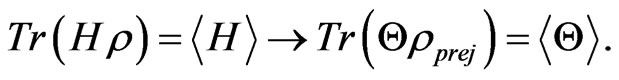(55)

In fact, if the density operator in quantum canonical system is given by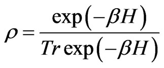, then using the similarity transformation one can obtain a projected density operator as

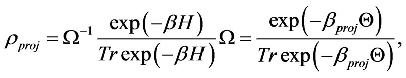(56)

which allows one to present (by extension) a new canonical ensemble distribution which is “vacuum” of “dynamic part” of the original, as expressed by Balescu’s book [25]

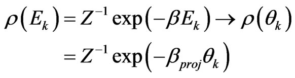(57)

with the partition functions as

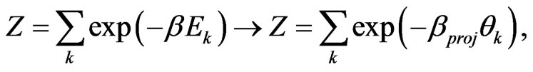(58)

where

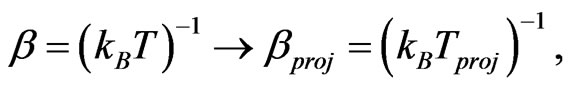
and is an eigenvalue of, is extended as function of position and time. This gives a precise formula of the quantum canonical ensemble for a projected density operator, which can be considered as generalizing the equilibrium quantum canonical ensembles formula to the non-equilibrium quantum canonical ensembles formula in the sense as 1) if the similarity operator is unitary, then the new formula is just an effective (or holographic) representation of the old equilibrium quantum canonical ensembles formula because or H has the same spectral structure, 2) if the similarity operator is non-unitary, then the new formula is an extension of the old formula, which represents kind of non-equilibrium quantum canonical ensembles formula and reflects irreversibility of the system. The spectrum of may appear to have complex spectral structure that is impossible to get from the original self-adjoint operator H in the Hilbert space, and 3) if the similarity operator can be deduced by some approximations, such as Markovian/non-markovian approximations, then the new formula can expose some non-equilibrium characteristics, which can not be gained from the equilibrium quantum ensemble formulas.

Thus it is obvious that the preceding constructed quantum formalism for density operator can be extended to the classical statistical canonical, grand canonical ensembles. Furthermore, the general canonical ensembles distribution can also be derived by using the similarity transformation. We want to emphasize again that in the book of Balescue [25] the “dynamic part” means essence part of (irreversible) evolution of the density distribution, and the “vacuum” means without correlations. His work and Brussels-Austin school late works seem to show that the plays an important or influential role in the (irreversible) evolution of the system by extending it to the Rigged Hilbert space or Rigged Liouville space [43,44]. Using this way can one build a corresponding relation between equilibrium statistical ensemble formalism and non-equilibrium statistical ensemble formalism? The answer is confirmed because the original Hamiltonian of the system has corresponding relation to the collision operator by the similarity transformation. Thus the dynamic variables Y are usually obtained by calculated over the non-equilibrium statistical distribution which is given by the proposed nonequilibrium statistical ensemble formulas (56) or (57) or solution of the SKE,. If the second order approximation of corresponds to the Master equation, the Boltzmann equation, the Pauli equation, or the Fokker-Planck equation, then should deliver the expectation of corresponding physical value in the non-equilibrium ensembles. The Equation (56) can be as starting base to get non-equilibrium statistical ensembles formulations for irreversibility.

As an application of the above formalism let us deduce the kinetic equations for the open system with strong coupling to the environment. In this case, it is not restricted whether system is Markovian or non-Markovian, but may be irreversible. Then we start directly from the SKE. Here we consider the case for the coupling is strong, since the model beyond the perturbation, which can not solved by usually equilibrium statistical method. Thus the kinetic equation is

(59)

where is a resolvent introduced as. Consider the eigenvalues problem and the Born series of expansion, and, one can get

(60)

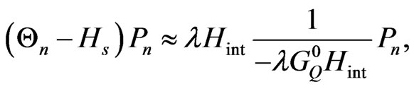
which gives the eigenvalues by

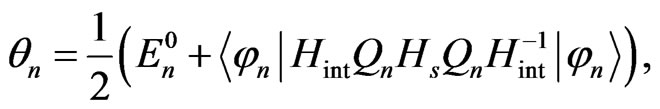(61)

hence, the density operator for this system can be obtained. For example, assume that a Hamiltonian for the Spin-Boson model is given by

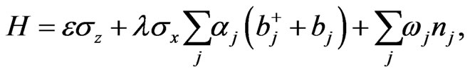(62)

where, belong to Pauli matrix, , and is a creation (a Boson, such as phonon or photon) operator for the Bosons of environment, and. Concerning with the eigenvectors of the free Hamiltonian are as, , , then the expansion of H with respect to the basis can be obtained. By introducing an eigen-projectorts as and, and considering Equation (59) and using the subdynamic procedure, one finally obtains, for, , which allows one easily to get a reduced density operator for the canonical system by

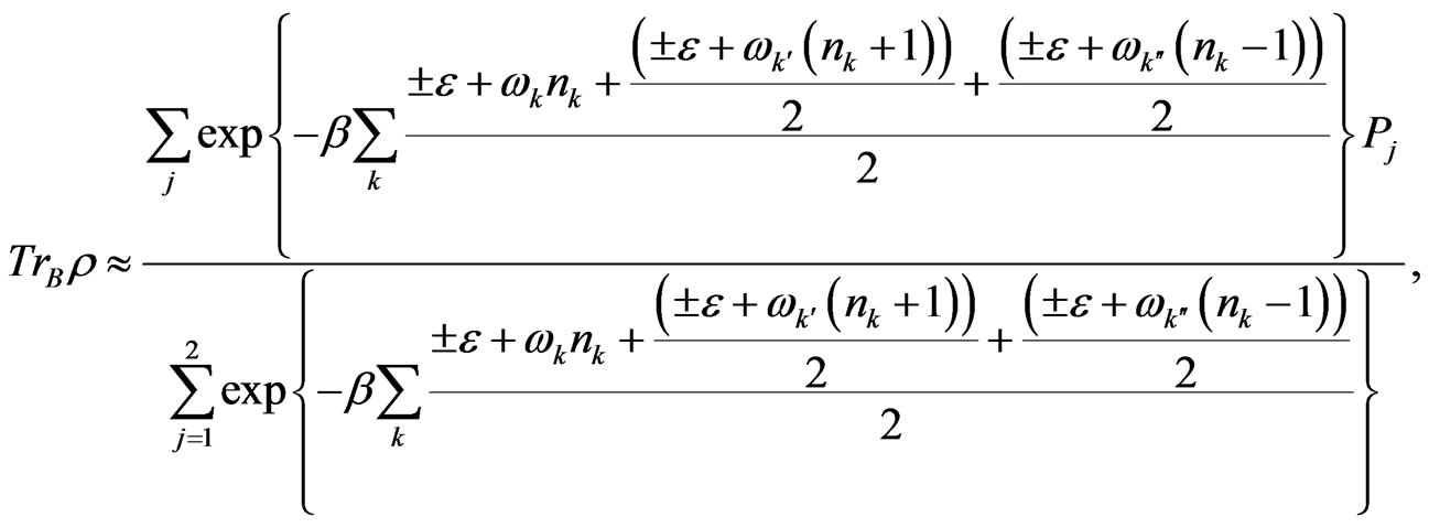(63)

where, select sign “+”, , select sign “−”. From Equation (63) one can easily see that the reduced density operator for the canonical system is independent upon the interaction part of Hamiltonian after final approximation, which means that the environment can not influence the system and the system is decoherence-free. Hence, the construction of the above system in the SKE subspace is quantum decoherence-free, which is useful for quantum computing.

6. Conclusion

The basic dyanmical equations are true to the QID; the transmission process of QID for the mutual information is related to dynamical evolution; the Liouville equations of QID intertwine with SKE of QID, which could establish a non-equilibrium statistical ensemble formalism and apply to control quantum decoherence by strongly coupling system. This exposes that quantum information is holographic through the similarity structure of subdynamic kinetic equations.

7. Acknowledgements

This work was supported by the grants from CIAEYZ2011-20, Chinese NSFC under the Grand No. 611 74151, and in Canada by NSERC, MITACS, CIPI, MMO, and CITO.

REFERENCES

- D. R. Simon, “On the Power of Quantum Computation,” SIAM Journal on Computing, Vol. 26, No. 5, 1997, pp. 1474-1483. doi:10.1137/S0097539796298637
- P. W. Shor, “Polynomial-Time Algorithms for Prime Factorization and Discrete Logarithms on a Quantum Computer,” SIAM Journal on Computing, Vol. 26, No. 5, 1997, pp. 1484-1509. doi:10.1137/S0097539795293172
- S. Wiesner, “Conjugate Coding,” SIGACT News, Vol. 15, No. 1, 1983, pp. 78-88. doi:10.1145/1008908.1008920
- C. Bennett, F. Bessette, G. Brassard, L. Salvail and J. Smolin, “Experimental Quantum Cryptography,” Journal of Cryptology, Vol. 5, No. 1, 1993, pp. 3-28. doi:10.1007/BF00191318
- P. W. Shor, “Algorithms for Quantum Computation: Discrete Logarithms and Factoring,” Proceedings of the 35th Annual Symposium on Foundations of Computer Science, Santa Fe, 1994, pp. 124-134. doi:10.1109/SFCS.1994.365700
- D. Deutch, “Quantum Computational Networks,” Proceedings of the Royal Society A, Vol. 425, No. 1868, 1985, pp. 73-90. doi:10.1098/rspa.1989.0099
- L. Grover, “A Fast Quantum Mechanical Algorithm for Database Search,” Proceedings of the 28th Annual ACM Symposium on the Theory of Computation, ACM Press, New York, 1995.
- S. Tomonaga, “On a Relativistically Invariant Formation of the Quantum Theory of Wave Fields, I.,” Progress of Theoretical Physics, Vol. 1, No. 2, 1946, pp. 27-42. doi:10.1143/PTP.1.27
- S. Tomonaga, “On a Relativistically Invariant Formation of the Quantum Theory of Wave Fields, II,” Progress of Theoretical Physics, Vol. 2, 1947, p. 101.
- H. P. Breuer, “The Theory of Quantum Open Systems,” Oxford University Press, New York, 2002.
- S. S. Schweber, “An Introduction to Relativistic Quantum Field Theory,” Row, Peterson and Company, Evanston, 1948.
- J. Schwinger, “Quantum Electrodynamics. I. A Covariant Formulation,” Physical Review, Vol. 74, No. 10, 1948, pp. 1439-1461. doi:10.1103/PhysRev.74.1439
- E. Prugovecki, “Principles of Quantum General Relativity,” World Scientific Publishing, Co. Pte. Ltd., Singapore City, 1995.
- D. Giulini, C. Kiefer and C. Lämmerzahl, “Quantum Gravity: From Theory to Experimental Search,” SpringerVerlag, New York, 2003.
- X. S. Xing, “On Dynamical Statistical Information Theory,” Transactions of Beijing Institute of Technology (Chinese), Vol. 24, 2004.
- B. Qiao, X. S. Xing and H. E. Ruda, “Dynamical Equations for Quantum Information and Application in Information Channel,” Chinese Physics Letters, Vol. 22, No. 7, 2005, p. 1618. doi:10.1088/0256-307X/22/7/016
- M. Ohya and D. Petz, “Quantum Entropy and Its Use,” Springer-Verlag/Heidelberg, Berlin/New York, 2004.
- H. J. Carmichael, “Statistical Methods in Quantum Optics 1, Master Equations and Fokker-Planck Equations,” Springer-Verlag/Heidelberg, Berlin/New York, 1999.
- C. Arndt, “Information Measures, Information and Its Description in Science and Engineering,” Springer-Verlag/Heidelberg, Berlin/New York, 2001.
- I. Antoniou and S. Tasaki, “Generalized Spectral Decompositions of Mixing Dynamical Systems,” International Journal of Quantum Chemistry, Vol. 46, No. 3, 1993, pp. 425-474. doi:10.1002/qua.560460311
- T. Petrosky and I. Prigogine, “Alternative Formulation of Classical and Quantum Dynamics for Non-Integrable Systems,” Physica A: Statistical Mechanics and Its Applications, Vol. 175, No. 1, 1991, pp. 146-209. doi:10.1016/0378-4371(91)90273-F
- I. Antoniou, Y. Melnikov and B. Qiao, “Master Equation for a Quantum System Driven by a Strong Periodic Field in the Quasienergy Representation,” Physica A: Statistical Mechanics and Its Applications, Vol. 246, No. 1-2, 1997, pp. 97-114. doi:10.1016/S0378-4371(97)00343-9
- B. Qiao, H. E. Ruda, M. S. Zhang and X. H. Zeng, “Kinetic Equation, Non-Perturbative Approach and Decoherence Free Subspace for Quantum Open System,” Physica A: Statistical Mechanics and Its Applications, Vol. 322, 2003, pp. 345-358. doi:10.1016/S0378-4371(02)01809-5
- B. Qiao, H. E. Ruda and Z. D. Zhou, “Dynamical Equations of Quantum Information and Gaussian Channel,” Physica A: Statistical Mechanics and Its Applications, Vol. 363, No. 2, 2006, pp. 198-210. doi:10.1016/j.physa.2005.08.044
- R. Balescu, “Equilibrium and Non-Equilibrium Statistical Mechanics,” Wiley, New York, 1975.
- S. Nakajima, “On Quantum Theory of Transport Phenomena,” Progress of Theoretical Physics, Vol. 20, No. 6, 1958, pp. 948-959. doi:10.1143/PTP.20.948
- R. Zwanzig, “Ensemble Method in the Theory of Irreversibility,” Journal of Chemical Physics, Vol. 33, No. 5, 1960, pp. 1338-1341. doi:10.1063/1.1731409
- S. Chapman, “Kinetic Theory of Simple and Composite Monatomic Gases: Viscosity, Thermal Conduction, and Diffusion,” Proceedings of the Royal Society of London. Series A, Vol. 93, No. 646, 1916, pp. 1-20. doi:10.1098/rspa.1916.0046
- D. Enskog, “Kinetische Theorie der Vorgäng in Mässig verdünnten Gasen,” Almqvist and Wiksells, Uppsala, 1917.
- N. N. Bogoliubov, “Kinetic Equations,” Journal of Physics-USSR, Vol. 10, No. 256, 1946, p. 265.
- M. Born and H. S. Green, “A General Kinetic Theory of Liquids,” Cambridge University Press, Cambridge, 1949.
- J. G. Kirkwood, “The Statistical Mechanical Theory of Transport Processes I. General Theory,” Journal of Chemical Physics, Vol. 14, No. 3, 1946, p. 180. doi:10.1063/1.1724117
- J. G. Kirkwood, “Selected Topics in Statistical Mechanics,” I. Oppenheim, Ed., Gordon and Breach, New York, 1967.
- J. Yvon, “La Theorie Statistiques des Fluides et l’Equation d’Etat, Herman et Cie, Paris, 1935.
- M. S. Green, “Markoff Random Processes and the Statistical Mechanics of Time—Dependent Phenomena. II. Irreversible Processes in Fluids,” Journal of Chemical Physics, Vol. 20, No. 3, 1954, pp. 398-413.
- R. Kubo, “Statistical-Mechanical Theory of Irreversible Processes. I. General Theory and Simple Applications to Magnetic and Conduction Problems,” Journal of the Physical Society of Japan, Vol. 12, 1957, pp. 570-586. doi:10.1143/JPSJ.12.570
- H. Mori, “Statistical-Mechanical Theory of Transport in Fluids,” Physical Review, Vol. 112, 1958, pp. 1829-1842. doi:10.1103/PhysRev.112.1829
- H. Mori, “Correlation Function Method for Transport Phenomena,” Physical Review, Vol. 115, 1959, pp. 298-300. doi:10.1103/PhysRev.115.298
- D. Zubarev, V. Morozov and G. Röpke, “Statistical Mechanics of Nonequilibrium Processes,” Akademie Verlag, Berlin, 1996.
- R. Luzzi, Á. R. Vasconcellos and J. G. Ramos, “Predictive Statistical Mechanics—A Non-Equilibrium Ensemble Formalism,” Kluwer Academic Publishers, Dordrecht, 2002.
- B. C. Eu, “Nonequilibrium Statistical Mechanics (Ensemble Method),” Kluwer Academic Publishers, Dordrecht/Boston/London, 1998.
- X. S. Xing, “On Non Equilibrium Statistical Physics— Concurrently on the Fundamental Equation of Nonequilibrium Entropy,” Scientia Sinica Physica, Mechanica & Astronomica, Vol. 40, No. 12, 2011, pp. 1441-1660.
- B. Qiao, H. E. Ruda, X. H. Zeng and B. B. Hu, “Extended Space for Quantum Cryptography Using Mixed States,” Physica A: Statistical Mechanics and Its Applications, Vol. 320, 2003, pp. 357-370. doi:10.1016/S0378-4371(02)01539-X
- B. Qiao, L. Guo and H. E. Ruda, “Quantum Computing in Decoherence-Free Subspace Constructed by Triangulation,” Advances in Mathematical Physics, Vol. 2010, 2010, Article ID: 365653.