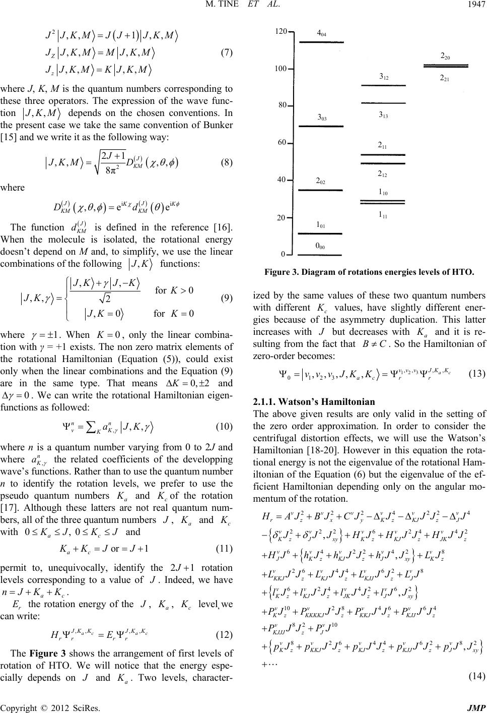
Journal of Modern Physics, 2012, 3, 1945-1957
http://dx.doi.org/10.4236/jmp.2012.312243 Published Online December 2012 (http://www.SciRP.org/journal/jmp)
Determination of the Vibro-Rotational Constants, the
Dipole Moment’s Function and the Intensities of the HTO’s
ν1 (ν3 by Usual Convention) Band
Modou Tine1, Diouma Kobor1, Ibrahima Sakho1, Laurent Coudert2
1Laboratoire de Chimie et de Physique des Matériaux (LCPM), Université de Ziguinchor, Ziguinchor, Sénégal
2Laboratoire Inter-Universitaire des Systèmes Atmosphériques, Créteil, France
Received June 29, 2012; revised October 16, 2012; accepted October 30, 2012
ABSTRACT
In the first part of this paper, an analysis of the high-resolution spectrum of the HTO molecule ν1(ν3) band, from 3630 to
3950 cm–1, was undertaken. The rotational transition of this band was assigned using combination differences. Their
wavenumbers were analyzed with a least squares fit program in order to obtain spectroscopic constants. A perturbed
state has been evidenced. In the second part, with a view towards building a spectroscopic data base, a calculation of the
dipolar momentum function was undertaken.
Keywords: Infrared Spectrum; Energy Level; Rays Intensities; Perturbation
1. Introduction
HTO molecule is important for the environment. It is
found in discharges of nuclear power plants with 12.3
years for half-life. It is essential to know its infrared
spectrum in order to detect it remotely. It is also interest-
ing to have available database to use this molecule spec-
troscopy. These were the motivation of our work focused
on the fundamental v1(v3) looks near 3700 cm–1.The aim
of this paper is twofold, firstly we perform a comprehen-
sive analysis of high-resolution spectrum of the v1(ν3)
band, and secondly we determine the dipole moment’s
function which will permit us to calculate the rays inten-
sities in a wide range of quantum numbers.
We continued with an analysis of the transitions wave
numbers to determine the spectroscopic constants that are
essential to calculate the positions of such transitions.
2. Theoretical Calculations
2.1. The Vibration-Rotation Hamiltonian
Leaving from the approximations of Born Oppenheimer
[1,2] and of the harmonic that consists in separating the
movement of the electrons to that of the cores and in de-
scribing the molecule while developing only the potential
energy to the second order, with the help of the 3N-6
correctly chosen coordinates. The vibration-rotation Ham-
iltonian, under compact shape, is written, according to
Darling and Dennison [3], simplified by Watson [4,5],
by:
 
 
2
1
1
2
1
2k
k
H
JP JP
PVQUQ

 



 



(1)
where the indices α and β correspond to the xyz axes of
the mobile reference mark. Jα and pα quantities are re-
spectively the components of the total angular moment
and the internal angular moment of the vibration; μαβ
represents the component of the efficient inertia tensor’s
inverse; pk with 136KN

 the conjugated momen-
tum of the normal coordinate of Qk vibration; V(Q) the
potential energy (quadratic) and U(Q) a term of a poten-
tial energy type. For the zero-order this Equation (1) be-
comes:
0vr
H
HH


With

322
1
1
2
vkk
k
H
PQ 


 (2)
By introducing the dimensionless normal coordinates,
we obtain:
14
12
k
kk
qQ

 and k
k
i
pq


The Equation (2) gets under the shape:

322
12
k
vkk
k
H
hcp q



 (3)

M. TINE ET AL. 1946
where
12
2π
k
kc

  is the k node energy in cm–1 and the c
constant, the light speed. The Equation (3) is the sum of
three harmonic oscillators. We deduce easily the wave’s
function as well as the vibrational energy:
 
3
123 1
,,
vvkk
k
vvvq



and
3
1
1
2
vk
k
Ehc v 





 (4)
where Φv(q) is the harmonic oscillator wave’s function
for the vibrational quantum number v. From this equation,
the values of the H2O, HDO and HTO three normal
nodes energies are given in the Table 1. The calculation
has been done taking into account the molecule geometry
at the equilibrium state and the surface potential energy
of Patridge and Schwenke [6]. To compare our results,
some energy levels, coming from the results of the ref-
erences [7-12], were presented in the same table. We
represented the small displacements to the H2O isitopic
in Figure 1. The normal modes are labeled using the
IUPAC convention [13], followed in brackets by the usual
convention. Hr can be written by:
2
r
HBJ



 (5)
where α corresponds to the x, y, z axes and

1
2
1
cm 8πe
h
BcI



r
H
has been calculated choosing the reference related
to the O’xyz molecule while the tensor of inertia would
be diagonal (Figure 2).
For an asymmetric molecule type, as HTO, the use is
to designate by A, B and C the constants of the rotational
Bα, with A > B > C. The corresponding axes have been
noted a, b, c.
Table 1. Calculated and observed energies of the three
normal modes for the isotopic varieties of water.
Variety Mode Calculated Observed
ν1 3831 3655
ν2 1648 1594
H2O
ν3 3942 3755
ν1 3889 3707
ν2 2824 2726
HDO
ν3 1445 1403
ν1 3888 3716
ν2 2369 1648
HTO
ν3 1370 1332
Figure 1. The small displacements of the three normal
nodes of vibration [13] of H2O, HDO and HTO.
B
z
H
A
O
Oʹ
T
x
Figure 2. The axes systems of HTO molecule.
Following the Ir representation


,,
x
by cza
the Equation (5) becomes :
 
 
222
22
22
11
22
1
4
rzxy
z
HAJBJCJ
A
BC JBCJ
BC JJ



  


 
(6)
where 2222
x
yz
J
JJJ

 and .
x
y
J
JiJ 
To estimate the molecule’s asymetry, we introduce the
Ray parameter [14] κ, equal to –0.8. This means that the
HTO molecule is enough close to a stretching asymmet-
ric rotator (1


).
There is no analytical forms for the eigenvalues of the
Equation (5). To obtain the rotation energy, it is neces-
sary to diagonalize the matrix of this hamiltonian in the
basis ,,
J
KM of the simultaneous eigenstates of the
total angular momentum
J
2 and of its projections on
the laboratory Z axis and the variable z of the mobile
reference, respectively, JZ and Jz.

M. TINE ET AL. 1947

2,,1 ,,
,, ,,
,, ,,
Z
z
J
JKMJ JJKM
J JKMMJKM
J JKMKJKM



(7)
where J, K, M is the quantum numbers corresponding to
these three operators. The expression of the wave func-
tion ,,
J
KM depends on the chosen conventions. In
the present case we take the same convention of Bunker
[15] and we write it as the following way:


2
21
,, ,,
8π
J
KM
J
JKM D



 (8)
where




ii
,, ee
JJ
K
K
KM KM
Dd


  
The function

J
K
M
d is defined in the reference [16].
When the molecule is isolated, the rotational energy
doesn’t depend on M and, to simplify, we use the linear
combinations of the following ,
J
K functions:
,,
for0
,, 2
,0for 0
JKJ KK
JK
JK K


 




(9)
where 1

 . When 0K, only the linear combina-
tion with γ = +1 exists. The non zero matrix elements of
the rotational Hamiltonian (Equation (5)), could exist
only when the linear combinations and the Equation (9)
are in the same type. That means 0, 2K and
0

. We can write the rotational Hamiltonian eigen-
functions as followed:
,,,
nn
vK
KaJK



 (10)
where n is a quantum number varying from 0 to 2J and
where ,
n
K
a

the related coefficients of the developping
wave’s functions. Rather than to use the quantum number
n to identify the rotation levels, we prefer to use the
pseudo quantum numbers a
K
and c
K
of the rotation
[17]. Although these latters are not real quantum num-
bers, all of the three quantum numbers
J
, a
K
and c
K
with 0,
a
K
J0c
K
J and
or 1
ac
KKJ J  (11)
permit to, unequivocally, identify the 21
J
 rotation
levels corresponding to a value of
J
. Indeed, we have
ac
nJKK .
r
E the rotation energy of the
J
, a
K
, c
K
level, we
can write:
,, ,,
ac ac
J
KK JKK
rr rr
HE (12)
The Figure 3 shows the arrangement of first levels of
rotation of HTO. We will notice that the energy espe-
cially depends on
J
and a
K
. Two levels, character-
120
100
80
60
40
20
0
2
02
3
03
4
04
1
01
0
00
1
10
1
11
2
12
2
11
3
13
3
12
2
20
2
21
Figure 3. Diagram of rotations energies levels of HTO.
ized by the same values of these two quantum numbers
with different c
K
values, have slightly different ener-
gies because of the asymmetry duplication. This latter
increases with
J
but decreases with a
K
and it is re-
sulting from the fact that BC. So the Hamiltonian of
zero-order becomes:
123
,,,,
0123
,,,, ,ac
vv vJKK
ac rr
vv v JKK  (13)
2.1.1. Watson’s Hamiltonian
The above given results are only valid in the setting of
the zero order approximation. In order to consider the
centrifugal distortion effects, we will use the Watson’s
Hamiltonian [18-20]. However in this equation the rota-
tional energy is not the eigenvalue of the rotational Ham-
iltonian of the Equation (6) but the eigenvalue of the ef-
ficient Hamiltonian depending only on the angular mo-
mentum of the rotation.


222 4224
2226 24 42
642242 8
264462 8
624426
,
,
vvvv vv
rzxyKzKJzJ
vvv vv
Kz JxyKzKJzJKz
vvv vv
JKzKJzJxyKz
vvvv
KKJz KJz KJJz J
vv v v
Kz KJz JKz J
HAJBJCJJJJ J
JJJHJHJJHJJ
HJhJ hJJ hJJLJ
LJJLJJ LJJLJ
lJ lJJ lJJ lJ

 
 
 

  


2
102 84 664
82 10
826446282
,
,
xy
vvv v
KzKKKKJ zKKJ zKJJ z
vv
KJJJz J
vvv vv
K
z KKJz KJ zKJJz Jxy
J
PJPJ JPJJPJ J
PJJ PJ
pJpJJpJJ pJJ pJJ


 

(14)

M. TINE ET AL. 1948
where 222
x
yxy
J
JJ and {,} is the ant-commutator as

,
A
BABBA.
In this equation, all parameters depend on the consid-
ered vibrationnal state as indicated by the exhibitor v.
The adopted resolution is the A-type which is more ade-
quate for an asymmetric molecule as HTO.
390 transitions have been assigned for J values below
15 (Table 2).
2.1.2. The Wave Numbers
For every transition, characterized by the rotationnal
quantum numbers ,,
ac
J
KK


and ,,
ac
J
KK
 for the
lower and higher levels, respectively, the wave number
cal

has been calculated by:

 
10
10
,,: ,,:
cal
racrac
vv
E
JK KPEJ KKP
EE

 

 (15)
Table 2. The transitions assigned in the infrared spectrum of the ν1(ν3) band of HTO.
J' a
K
 c
K
 J" a
K

 c
K

 Obs Cal Diff
2
1
6
3
2
5
5
0
4
5
5
1
8
1
4
1
3
3
2
11
11
2
6
10
10
10
10
9
9
9
9
8
8
1
8
8
6
6
6
6
5
5
4
9
9
8
7
7
6
6
5
5
2
0
1
1
1
0
2
0
0
1
2
1
2
0
2
1
0
1
1
5
5
0
2
5
5
6
6
6
6
5
5
6
6
0
5
5
6
6
5
5
5
5
1
3
4
4
4
4
4
4
4
4
1
1
6
3
2
5
4
0
4
5
3
0
7
1
3
1
3
3
2
7
6
2
5
6
5
5
4
4
3
5
5
3
2
1
4
3
0
1
1
2
0
1
4
7
5
5
4
3
2
3
1
2
3
2
6
4
3
5
4
1
4
5
4
2
8
2
5
2
3
2
3
11
11
2
5
10
10
10
10
9
9
9
9
8
8
1
8
8
6
6
6
6
5
5
3
9
9
8
7
7
6
6
5
5
2
1
1
0
1
1
3
1
1
1
3
1
2
0
1
1
1
2
0
5
5
1
3
5
5
6
6
6
6
5
5
6
6
1
5
5
6
6
5
5
5
5
2
3
4
4
4
4
4
4
4
4
2
2
5
4
3
4
1
1
3
4
2
1
6
2
4
2
2
0
3
6
7
1
2
5
6
4
5
3
4
4
5
2
3
0
3
4
1
0
2
1
1
0
1
6
6
4
3
4
3
2
2
1
3678.521(10)
3678.849(10)
3680.963(10)
3682.342(10)
3683.105(10)
3683.710(10)
3686.775(10)
3688.956(10)
3689.717(10)
3690.777(10)
3690.777(50)
3690.937(10)
3691.777(10)
3693.354(10)
3693.994(10)
3694.065(50)
3694.102(10)
3694.970(10)
3695.623(10)
3696.543(10)
3696.643(10)
3697.093(10)
3697.172(10)
3697.518(10)
3697.518(10)
3697.708(10)
3697.708(10)
3698.242(10)
3698.242(10)
3698.360(10)
3698.360(10)
3698.658(10)
3698.658(10)
3698.941(10)
3699.149(10)
3699.149(10)
3699.524(10)
3699.524(10)
3700.508(10)
3700.508(10)
3701.061(10)
3701.061(10)
3702.410(50)
3702.935(10)
3702.935(10)
3703.183(10)
3703.817(10)
3703.879(10)
3704.358(50)
3704.358(50)
3704.817(10)
3704.817(10)
3721.521
3658.849
3692.963
3704.342
3696.105
3669.710
3549.775
3660.956
3687.717
3698.777
3714.777
3693.937
4057.777
3679.354
3603.994
3688.065
3686.102
3694.970
3695.623
3678.543
3680.643
3680.093
3392.172
3665.518
3703.518
3714.708
3715.708
3655.242
3655.242
3693.360
3703.360
3719.658
3719.658
3665.941
3699.149
3702.149
3702.524
3702.524
3697.508
3697.508
3694.061
3694.061
3694.410
3718.935
3664.935
3699.183
3709.817
3711.879
3738.358
3720.358
3731.817
3727.817
−43
20
−12
−22
−13
14
137*
28
2
−8
−24
−3
−362*
14
90*
6
8
0
0
18
16
17
305*
32
−6
−17
−18
43
43
5
−5
−21
−21
33
0
−3
−3
−3
3
3
7
7
8
−16
38
4
−6
−8
−34
−16
−27
−23
6 2 4 5 3 3 3704.817(50) 3733.817 −29

M. TINE ET AL. 1949
Continued
3
0
4
4
6
8
3
7
5
6
1
5
1
0
4
4
2
3
1
3
1
3
1
2
2
0
0
1
5
6
3
5
5
4
1
4
2
1
4
4
6
8
3
7
4
6
2
5
2
0
4
4
2
3
1
3
2
3
0
2
1
1
1
0
4
5
2
4
2
3
2
3
3704.857(50)
3704.939(50)
3705.197(10)
3705.197(10)
3705.219(10)
3705.518(10)
3705.744(50)
3707.199(10)
3708.150(50)
3708.254(10)
3708.554(10)
3708.930(50)
3722.857
3684.939
3676.197
3734.197
3417.219
3714.518
3724.744
3713.199
3705.150
3723.254
3724.554
3584.930
−18
20
29
−29
288*
−9
−19
−6
3
−15
−16
124*
5
6
4
4
3
3
8
2
4
6
3
2
2
3
1
4
5
5
1
4
4
6
2
2
2
7
3
1
8
4
4
1
5
2
4
3
2
3
5
2
2
4
1
5
6
3
3
3
4
6
3
3
2
6
6
7
3
3
3
3
3
3
3
1
2
1
2
2
2
2
1
2
2
2
1
1
2
2
1
0
2
2
1
0
2
1
3
1
1
1
3
0
1
1
1
0
1
1
1
1
1
1
2
2
0
1
0
1
1
1
2
2
3
3
2
1
1
0
5
2
3
6
2
1
0
1
1
2
3
3
0
3
2
4
1
2
1
5
2
1
6
3
2
0
4
1
1
3
2
2
4
2
1
3
1
4
5
3
2
1
4
5
3
2
2
5
4
5
5
6
4
4
3
3
8
2
4
5
3
2
2
3
1
4
5
5
1
3
5
6
2
1
3
7
3
0
8
4
5
1
4
2
5
2
1
3
5
1
1
4
0
5
6
2
2
2
3
5
2
2
1
6
6
7
3
3
3
3
3
3
3
1
2
2
2
2
2
2
1
2
2
2
1
2
1
2
1
1
1
2
1
0
2
1
2
0
2
0
2
1
1
0
1
0
1
0
0
0
1
1
2
2
1
2
0
1
0
0
1
1
2
4
1
2
0
1
6
1
2
3
1
0
1
2
0
3
4
4
1
2
5
5
2
1
2
6
3
0
7
4
3
1
3
2
4
2
1
3
5
1
0
4
0
5
6
2
1
0
3
4
2
1
1
6
5
6
3708.930(50)
3709.119(10)
3709.373(10)
3709.430(50)
3709.685(50)
3709.695(50)
3710.114(10)
3710.775(10)
3711.338(10)
3711.866(50)
3712.651(10)
3713.257(50)
3713.496(10)
3713.832(50)
3714.137(10)
3714.756(10)
3716.657(10)
3716.657(10)
3717.367(10)
3719.221(10)
3719.327(10)
3719.865(10)
3720.452(50)
3723.518(10)
3724.079(10)
3724.568(10)
3725.042(10)
3728.149(10)
3730.842(10)
3731.131(10)
3721.577(10)
3733.357(10)
3734.056(10)
3734.942(50)
3735.299(50)
3736.028(10)
3737.204(10)
3737.549(10)
3738.615(10)
3739.500(10)
3740.513(10)
3741.318(50)
3743.338(10)
3746.505(10)
3747.373(10)
3747.668(10)
3748.046(10)
3748.544(10)
3748.608(10)
3749.199(10)
3750.541(10)
3752.710(10)
3753.185(10)
3753.185(50)
3754.397(10)
3754.468(10)
3720.930
3744.119
3716.373
3734.430
3700.685
3701.695
3737.114
3722.775
3638.338
3672.866
3699.257
3742.257
3739.496
3694.832
3714.137
3685.756
3692.657
3692.657
3709.367
3728.221
3692.327
3700.865
3713.452
3698.518
3725.079
3716.568
3735.042
3712.149
3718.842
3740.131
3693.577
3725.357
3735.056
3748.942
3723.299
3719.028
3737.204
3744.549
3753.615
3723.500
3750.513
3770.318
3747.338
3762.505
3765.373
3759.668
3725.046
3738.544
3739.608
3755.199
3732.541
3764.710
3763.185
3753.185
3742.397
3754.468
−12
−35
−7
−25
9
8
−27
−12
73*
39
13
−29
−26
19
0
29
24
24
8
−9
27
19
7
25
−1
8
−10
36
12
−9
28
8
−1
−14
12
17
0
−7
−15
16
−10
−29
−4
−16
−18
−12
23
10
9
−6
18
−12
−10
0
12
0
5 2 3 5 1 4 3755.434(10) 3730.434 25

M. TINE ET AL. 1950
Continued
8
4
4
4
4
9
3
2
3
3
2
1
2
2
6
2
1
2
4
9
1
8
3
3
4
3
7
3
1
3
3
1
1
1
1
7
1
0
3
3
8
2
3755.919(10)
3755.994(50)
3756.024(50)
3757.218(10)
3757.948(10)
3758.901(10)
3759.322(50)
3746.919
3740.994
3746.024
3735.218
3773.948
3850.901
3764.322
9
15
8
22
−16
8
−5
4
4
5
4
7
2
3
5
5
10
7
4
2
5
5
5
3
6
6
11
4
5
8
5
4
10
5
6
6
6
5
9
5
12
6
5
6
6
6
8
6
7
7
6
7
7
6
6
2
6
7
2
6
5
7
7
4
4
3
5
7
6
8
7
2
2
0
0
1
2
1
4
4
2
1
1
2
3
3
1
2
5
5
3
1
2
1
0
2
3
2
0
4
4
2
3
1
2
1
1
3
3
2
3
0
5
5
2
3
0
2
1
2
3
1
2
1
3
0
3
3
3
3
3
1
3
0
3
3
2
5
4
6
0
3
1
2
8
6
3
1
3
2
5
2
2
1
8
4
4
7
5
3
7
3
6
2
3
4
6
4
10
6
5
4
3
5
5
6
3
2
5
4
7
4
6
1
3
7
0
5
2
7
4
1
2
1
3
7
4
8
5
3
3
4
3
7
2
2
4
4
10
6
3
2
4
4
4
3
5
5
11
3
4
8
4
4
10
4
5
5
5
5
9
4
12
5
4
5
5
6
8
5
6
6
5
7
6
5
5
1
6
6
1
5
5
6
6
4
4
3
5
6
6
7
7
2
2
1
0
0
1
0
4
4
1
2
1
1
3
3
1
1
5
5
2
0
2
0
0
1
2
2
1
4
4
1
2
1
1
1
0
3
3
1
2
0
5
5
2
2
1
2
0
1
2
1
1
1
2
0
3
2
2
2
2
0
2
1
2
2
1
4
3
7
1
2
0
1
9
5
2
2
2
1
4
3
1
0
9
3
3
8
4
4
8
2
5
1
2
5
7
3
11
5
4
3
2
6
6
5
2
1
4
5
6
3
5
0
4
6
1
4
3
6
3
2
3
2
4
6
5
7
6
3759.322(50)
3760.535(10)
3760.953(10)
3761.107(10)
3761.276(10)
3761.348(10)
3762.176(10)
3762.870(10)
3762.870(10)
3763.546(10)
3764.473(10)
3764.730(10)
3765.979(10)
3767.325(10)
3765.453(10)
3768.021(10)
3768.228(10)
3769.881(10)
3769.881(10)
3770.189(10)
3770.439(50)
3770.439(50)
3770.593(10)
3771.163(10)
3771.245(10)
3772.669(10)
3772.777(10)
3772.819(10)
3774.061(10)
3774.061(10)
3775.010(10)
3776.061(10)
3776.516(10)
3777.718(10)
3777.858(10)
3778.226(10)
3778.610(10)
3778.950(10)
3779.601(10)
3779.904(10)
3780.716(10)
3780.874(10)
3780.874(10)
3781.421(10)
3783.693(10)
3784.088(10)
3785.251(10)
3785.755(10)
3786.069(10)
3787.024(10)
3787.478(10)
3787.775(10)
3787.963(10)
3789.632(10)
3789.883(10)
3790.601(10)
3791.438(10)
3793.025(10)
3793.088(10)
3793.165(10)
3793.274(10)
3793.617(10)
3794.388(10)
3794.499(10)
3676.322
3743.535
3748.953
3757.107
3770.276
3783.348
3778.176
3780.870
3776.870
3749.546
3763.473
3779.730
3783.979
3773.325
3774.453
3777.021
3740.228
3805.881
3805.881
3762.189
3799.439
3601.439
3768.593
3756.163
3675.245
3781.669
3779.777
3734.819
3800.061
3791.061
3608.010
3793.061
3786.516
3765.718
3781.858
3789.226
3789.610
3801.950
3450.601
3794.904
3735.716
3778.874
3778.874
3446.421
3802.693
3677.088
3770.251
3784.755
3793.069
3800.024
3767.478
3809.775
3805.963
3789.632
3680.883
3802.601
3777.601
3781.025
3763.088
3791.165
3770.274
3796.617
3653.388
3793.499
83*
17
12
4
− 9
−22
−16
−18
−16
14
1
−15
−18
−6
−9
−9
28
−36
−36
8
−29
169*
2
15
96*
−9
7
38
−26
−17
167*
−17
−10
12
−4
−11
−11
−23
329*
−15
45
2
2
335*
−19
107*
15
1
−7
−13
20
−22
−18
0
109*
−12
14
12
30
2
23
−3
141*
1

M. TINE ET AL. 1951
where i
v
E is the vibrationnal energy of the i state and

,, :
i
rac
EJKK P represents the rotational energy of
the J, Ka, Kc level, calculated with the efficient Hamilto-
nian given by the Equation (14) for the i P spectro-
scopic parameter of the i vibrationnal state.
In this work, the 0 P spectroscopic parameters of the
fundamental state have been considered equal to the
Helminger’s values published in [21] and 0
v
E arbitrarily
fixed at zero. The 1
P spectroscopic parameters of the
vibrationnal state v1 = 1 has been determined by adjust-
ment using the least squares program. The results of the
analysis are in the Tables 2 and 3.
2.2. The ν1(ν3) Band Intensity
To calculate the transitions intensity, it is necessary for
us to determine, at first, the dipolar momentum function.
2.2.1. Determination of the Dipolar Momentum
Function
From the S1 and S2 coordinates corresponding respec-
tively to the following small variations ∆r31 and ∆r32 of
the inter atomic distances and S3 corresponding to small
variations of the valence angle ∆Φ, the Schrödinger
equation for the vibration [22] becomes:
33
,1 ,1
11
22
vijijijij
ij ij
H
GPPFSS



(16)
where i
i
i
PS




is the conjugated momentum of the co-
ordinate i
S, G and F correspond respectively to the
kinetic and potential energies and can be calculated nu-
merically from the Wilson Equation [22] once the mole-
cule’s equilibrium configuration is known. The F tensor
components can be calculated numerically using Patridge
and Schwenke [6] potential energy surface. The v
H
eigenenergies were obtained by solving the following
equation:
1
F
XGX 

 (17)
where

and X are respectively eigenvalue and ei-
genvector.
Thus we can deduce the equation permitting the pas-
sage from normal dimensionless coordinates k q to the
internal coordinates.
3
14 1
k
i
ik
k
k
X
Sq





 (18)
Then we try to obtain the dipolar momentum function
according to the internal coordinates:
3
0
1
ssi
x
xxi
iS
 



and
3
0
1
ssi
z
zzi
iS
 


 (19)
Table 3. The spectroscopic constants of the fundamental and the v1(v3) band of HTO.
Constant value to the ν1(ν3) band Constant value to the fundamental
E1 3716.5475(48) E0 0
A
B
C
21.8482(37)
6.58908(75)
4.97656(72)
A
B
C
22.61061
6.61116
5.01889
∆K
∆KJ
∆J
δK
δJ
13.796(810) × 10–3
2.306(130) × 10–3
0.1628(71) × 10–3
–6.710(320) × 10–3
16.670(390) × 10–6
∆K
∆KJ
∆J
δK
δJ
9.04872 × 10–3
1.61856 × 10–3
0.17385 × 10–3
1.71208 × 10–3
47.1697 × 10–6
HK
HKJ
HJK
HJ
hK
hKJ
hJ
888.900(680) × 10–6
127.500(160) × 10–6
–24.000(18) × 10–6
–0.224(64) × 10–6
–894.900(360 × 10–6
–35.500(270) × 10–6
–0.140(16) × 10–6
HK
HKJ
HJK
HJ
hK
hKJ
hJ
29.880 × 10–6
–2.110 × 10–6
1.316 × 10–6
17.337 × 10–9
17.947 × 10–6
0.5713 × 10–6
5.946 × 10–9
LK
LKKJ
LKJ
–0.277 × 10–6
0.0659 × 10–6
–0.018 × 10–6
lK
lKJ
–0.2713 × 10–6
–3.0395 × 10–9
PK 3.673 × 10–9
LK
LKKJ
LKJ
LKJJ
LJ
IK
IKJ
IJK
PK
PKKKJ
pK
–20.000(24) × 10–6
–11.130(50) × 10–6
1.906(120) × 10–6
0.0831(90) × 10–6
0.404(180) × 10–9
29.781(1600) × 10–6
0.924(80) × 10–6
89.840(760) × 10–9
238.400(300) × 10–9
115.200(100) × 10–9
–196.900(150) × 10–9
pK 0.969 × 10–9

M. TINE ET AL. 1952
where 0s


with or
x
z

 and
s
i


with 13i


are constants.
To determine the HTO dipolar momentum function,
we use the unvariability of this function with an isotopic
substitution when it is expressed by the internal coordi-
nates. However, it will be necessary to take to account
the way from which the molecule depending reference
mark O’xyz is going to change.
From the Equation (18) and by replacing the Si by the
qi in the Equation (19), we find the HTO dipolar mo-
mentum function expressed in the normal dimensionless
coordinates. Considering the Equation (18), the terms
k
i
X
and k

will have the values corresponding to the
HTO normal modes and the results are shown in the Ta-
ble 4.
2.2.2. The Absorption Band Intensity
The intensity of a molecular absorption band, in a gas at
the thermodynamic equilibrium [23], is given as fol-
lowed:
3
36
2
8π10 exp
3
1exp
BAAB A
A
AB
Z
g
hcE
ShcQ KT
hc AB
KT









 
 


(20)
where
B
A
S is the intensity in cm–1/(molécule·cm–2) for a
transition from the lower level A to the up level B at the
T temperature; A
g
is the degenerancy due to the nu-
clear spin of the lower level A; AB

is the transition
wave number in cm–1;
A
E is the lower energy level in 1 cm; Q the distribu-
tion’s function; K the Boltzmann’s constant and
Z


is
the modified transition momentum in Debye. Its expres-
sion [23] is:
Z
xx zz


 (21)
where
x

and
z

are the dipolar momentum compo-
nents, in the reference mark related to the molecule, ex-
pressed according to the normal dimensionless coordi-
nates.
x
 and
z
 are operators [23] depending to the
vibrational coordinates which matrix elements are given
in the Tables 5 and 6.
From the Tables 3 and 5, the wave number and the
Table 4. Thevalues of the coefficients used in the develop-
ment of the dipolar momentum function.
Coefficients Valeur Coefficients Valeur
0
x

–1.74117 0
z

–0.84923
1
x

× 21/2 –0.01060 1
z

× 21/2 –0.03502
2
x

× 21/2 0.10583 2
z

× 21/2 –0.05269
3
x

× 21/2 –0.03039 3
z

× 21/2 0.04091
intensity of the authorized transitions have been calcu-
lated using Equations (15) and (20), for 11J

, for a
temperature of 296 K.
The Table 7 gives the portion of list covering the re-
gion 3630 to 3760 cm–1 for the transitions which inten-
sity is over


23 12
10cmmolecule cm
 
.
3. Results and Discussion
3.1. Analysis of Waves Numbers
In this analysis, the efficient hamiltonian spectroscopic
parameters of the Equation (14) and the vibrational en-
ergy have been considered.
The mean quadratic gap q = 0.018 cm–1 is enough
close to the experimental one for the observed wave
number: 0.010 cm–1. It is also possible to evaluate the
quality of the analysis with the standard deviation σ = 1.7.
Ideally, this value should be very close to 1. This excess
can be the consequence of the underestimation of the
experimental uncertainties and the use of an unadequate
efficient Hamiltonian. In this latter, it can come from a
perturbation of the superior vibrationnal state. This hy-
pothesis is confirmed by the results in the Table 2 for the
transitions presenting a big gap (Obs.-Cal.) or even those
that have been excluded in the analysis (in asterisk in the
Table 2).
One realizes that these transitions often share the same
superior rotationnal level and that the gap (Obs.-Cal.) is
practically independent of the low level.
The Table 8 illustrates well this fact for transitions ex-
cluded in the analysis for which the superior rotationnal
levels are 808 and 625.
Presumably, the vibrationnal state v1 = 1 is not isolated.
It exists another closed vibrationnal state which is cou-
pled whith it. To make a correct calculation of the vibra-
tionnal energy, it would be necessary to treat simultane-
ously these two states. A calculation based on Table 1
Table 5. The non zero elements matrix [23] operator Φz.
∆J ∆K Γ , , , ,
z
JKJ K


 
0 0




12
21 1KJ JJ 

±1 0




12
22
–Km Km


Table 6. The non zero elements matrix [23] operator Φx.
∆J∆KΓ , , , ,
z
JKJ K




0±1





12
121 11
2JJKKJKKJJ 

±1 ±1




12
11
2JKm KKmKKm

  



M. TINE ET AL. 1953
Table 7. Waves numbers and lines intensities of v1(v3) band of HTO.
J' a
K
 c
K
 J" a
K

 c
K

 Cal S
2
2
1
7
2
9
3
5
11
7
10
11
8
5
8
0
10
9
4
5
5
1
11
8
8
11
4
1
9
11
4
1
3
3
2
8
8
8
11
11
6
2
9
11
11
10
10
10
10
9
9
9
9
9
9
9
9
8
8
1
2
0
1
1
2
0
0
4
3
3
4
3
2
3
0
4
3
0
1
2
1
0
2
1
1
0
0
4
3
2
1
0
1
1
3
8
8
5
5
2
0
3
6
6
5
5
6
6
6
6
8
8
5
5
9
9
6
6
1
1
1
6
2
8
3
5
8
5
7
7
6
4
5
0
6
6
4
5
3
0
11
7
7
11
4
1
6
9
3
1
3
3
2
5
1
0
7
6
5
2
7
6
5
6
5
5
4
4
3
2
1
5
4
0
1
3
2
3
3
2
6
3
9
2
5
10
8
11
10
7
4
7
1
11
10
4
5
4
2
10
8
7
10
3
2
10
11
5
2
3
2
3
9
9
9
11
11
5
2
8
11
11
10
10
10
10
9
9
10
10
9
9
10
10
8
8
1
2
1
3
1
2
2
1
5
2
2
5
4
3
4
1
3
2
1
1
3
1
2
2
3
2
2
0
3
3
1
1
1
2
0
2
8
8
5
5
3
1
4
6
6
5
5
6
6
6
6
8
8
5
5
10
10
6
6
2
2
2
3
3
7
0
4
5
6
10
6
3
1
4
1
9
9
3
4
2
1
8
6
4
8
1
2
7
8
4
2
2
0
3
5
2
1
6
7
2
1
4
5
6
5
6
4
5
3
4
3
2
4
5
1
0
2
3
3678.528
3678.564
3678.828
3679.121
3683.118
3683.043
3683.299
3683.695
3684.293
3684.665
3685.350
3685.575
3685.976
3686.796
3688.519
3688.927
3689.439
3689.711
3689.714
3690.785
3690.802
3690.941
3692.047
3691.788
3692.310
3692.615
3693.035
3693.340
3693.679
3693.883
3693.985
3694.058
3694.093
3694.968
3695.622
3696.172
3696.388
3696.388
3696.552
3696.653
3697.186
3697.075
3697.116
3697.356
3697.359
3697.498
3697.537
3697.724
3697.725
3698.201
3698.201
3698.205
3698.205
3698.358
3698.371
3698.568
3698.568
3698.679
3698.679
6.47e−20
3.24e−20
2.22e−19
1.00e−22
6.79e−20
1.34e−21
7.21e−23
2.59e−19
1.31e−21
1.67e−20
2.63e−21
1.31e−21
6.99e−21
1.60e−20
7.03e−21
1.65e−19
2.45e−21
5.18e−21
3.32e−19
5.34e−21
1.65e−20
4.38e−20
3.26e−21
2.66e−21
1.28e−22
9.26e−22
2.21e−22
6.41e−20
4.01e−21
5.50e−22
5.86e−20
4.49e−20
3.70e−19
1.73e−20
1.67e−19
8.99e−21
3.63e−23
3.63e−23
5.29e−22
5.29e−22
1.96e−20
3.45e−19
5.87e−21
3.24e−22
3.24e−22
1.08e−21
1.08e−21
6.62e−22
6.62e−22
1.29e−21
1.29e−21
3.99e−23
3.99e−23
2.11e−21
2.11e−21
2.66e−23
2.66e−23
2.39e−21
2.39e−21
1
4
7
7
0
1
6
6
1
4
2
1
1
4
7
7
1
1
6
6
0
3
1
2
3698.907
3699.079
3699.123
3699.123
2.46e−19
8.72e−21
4.26e−21
4.26e−21

M. TINE ET AL. 1954
Continued
8
7
7
11
6
6
10
5
5
5
9
6
10
10
9
4
9
11
10
9
9
8
8
7
7
9
7
6
6
5
5
6
3
0
6
4
4
8
9
3
7
9
6
10
10
7
9
10
5
6
1
5
5
8
6
5
3
7
4
4
8
7
3
3
3
5
5
5
4
5
5
0
5
5
0
4
3
1
4
3
1
4
4
4
4
3
4
4
4
4
1
3
4
4
4
4
2
1
0
2
4
4
3
3
1
2
0
0
8
8
3
1
3
1
3
1
2
3
4
3
3
2
3
3
3
0
0
3
3
3
4
3
2
8
2
1
10
1
0
5
5
4
10
7
6
4
6
7
6
5
7
5
4
4
3
8
4
3
2
2
1
4
2
0
5
1
0
6
6
3
6
9
6
3
2
5
9
8
5
4
1
4
3
5
3
2
2
4
2
1
8
7
1
0
0
8
7
7
11
6
6
9
5
5
4
10
7
9
10
8
3
9
11
10
9
9
8
8
7
7
8
8
6
6
5
5
5
2
1
6
4
4
8
10
3
6
8
5
11
11
7
8
9
4
6
2
5
5
9
6
5
4
7
4
4
7
6
3
3
3
5
5
5
4
5
5
2
5
5
2
3
2
2
4
4
2
4
4
4
4
3
4
4
4
4
3
2
4
4
4
4
3
2
0
2
4
4
3
1
1
3
2
2
8
8
3
2
4
2
3
0
2
3
3
3
3
1
3
3
3
2
2
3
3
3
3
2
3
7
1
2
7
0
1
2
8
5
7
6
5
1
5
8
7
6
6
4
5
3
4
5
7
2
3
1
2
3
1
1
4
0
1
5
9
2
3
6
3
4
3
4
6
5
2
3
2
3
2
6
5
3
3
5
1
2
5
4
0
1
1
3699.147
3699.863
3699.864
3700.237
3700.500
3700.500
3700.500
3701.048
3701.048
3701.056
3701.063
3701.368
3701.418
3701.470
3701.986
3702.401
3702.414
3702.529
3702.573
3702.899
3702.953
3703.180
3703.370
3703.825
3703.889
3703.941
3704.346
3704.376
3704.393
3704.842
3704.845
3704.847
3704.876
3704.918
3705.251
3705.227
3705.227
3705.528
3705.534
3705.763
3706.308
3706.420
3706.744
3706.895
3706.895
3707.206
3707.885
3707.903
3708.146
3708.269
3708.570
3708.964
3708.943
3709.016
3709.155
3709.242
3709.316
3709.370
3709.380
3709.456
3709.349
3709.746
3709.676
3709.687
3709.687
3.94e−21
7.03e−21
7.03e−21
6.63e−22
1.21e−21
1.21e−20
7.10e−21
2.00e−20
2.00e−20
3.72e−22
3.95e−21
2.00e−20
2.13e−21
1.38e−21
5.92e−21
2.87e−20
2.72e−21
6.65e−22
1.38e−21
2.72e−21
2.47e−21
5.10e−21
5.10e−21
9.14e−21
9.14e−21
1.34e−22
1.36e−20
1.57e−20
1.57e−20
2.62e−20
2.62e−20
2.09e−20
2.33e−20
3.60e−20
9.30e−21
4.28e−20
4.28e−20
4.79e−21
1.63e−23
1.43e−20
1.90e−20
1.41e−22
4.28e−22
3.13e−23
3.13e−23
8.77e−21
4.60e−21
4.37e−21
3.01e−20
1.53e−20
9.17e−20
1.62e−20
2.57e−20
5.76e−21
1.53e−20
2.57e−20
4.58e−20
8.78e−21
4.21e−20
4.21e−20
2.48e−22
3.66e−22
6.87e−20
6.87e−20
6.87e−20

M. TINE ET AL. 1955
Continued
8
2
4
9
8
6
6
3
7
7
8
2
7
7
10
10
2
3
6
1
10
10
8
4
5
8
8
8
7
10
8
5
6
5
8
1
11
9
9
11
4
4
6
7
11
9
2
5
9
10
10
7
2
2
5
7
3
7
3
10
9
4
10
3
1
2
3
1
1
2
2
2
1
4
2
7
7
1
5
2
2
3
1
5
3
2
2
2
7
7
2
2
3
3
2
2
3
2
1
3
7
7
3
1
2
2
2
1
2
1
2
2
7
7
4
0
2
3
2
1
4
2
2
5
2
2
5
2
3
6
8
6
4
2
5
7
4
1
1
0
9
6
0
1
3
1
5
7
7
2
3
2
1
6
5
7
5
3
4
3
6
0
9
3
2
8
3
2
4
5
10
7
1
3
8
4
3
4
2
1
2
5
2
3
1
9
5
2
8
8
2
4
9
7
5
7
3
8
6
9
2
7
7
9
11
2
3
7
1
11
10
7
4
6
8
8
9
8
9
9
5
7
6
9
1
10
9
9
11
3
5
6
6
10
10
2
6
8
10
10
8
1
3
6
7
3
8
4
9
10
5
11
3
1
2
3
2
2
1
2
1
2
3
2
7
7
3
4
2
2
2
1
4
3
3
2
1
7
7
1
0
4
1
2
0
2
0
1
4
7
7
3
2
1
2
3
3
1
1
0
3
7
7
3
1
1
2
2
1
3
1
3
4
0
1
6
1
2
7
5
3
7
1
8
4
7
0
0
1
6
7
1
2
6
0
8
8
4
3
6
1
2
9
8
6
8
4
7
4
9
1
6
2
3
9
2
5
5
4
7
10
2
6
5
3
4
5
1
2
5
6
2
6
4
6
6
5
11
3710.140
3710.787
3711.346
3711.777
3711.699
3711.826
3712.596
3712.637
3712.803
3713.116
3713.161
3713.286
3713.305
3713.305
3713.361
3713.442
3713.523
3713.812
3713.825
3714.137
3714.491
3714.599
3714.328
3714.727
3714.819
3715.312
3715.312
3715.443
3715.547
3716.434
3716.471
3716.633
3716.660
3717.007
3717.241
3717.358
3718.141
3718.468
3718.468
3718.865
3719.231
3719.300
3719.846
3719.889
3719.979
3720.385
3720.445
3720.612
3721.537
3723.159
3723.159
3723.377
3723.493
3724.080
3724.242
3724.560
3725.053
3725.511
3725.722
3726.797
3727.181
3727.190
3727.394
4.81e−21
2.45e−20
2.74e−20
2.50e−21
9.11e−21
2.42e−20
1.30e−20
4.53e−20
7.01e−21
1.60e−20
5.72e−21
7.74e−20
2.10e−21
2.10e−21
1.15e−22
1.14e−21
7.74e−20
4.54e−20
1.79e−20
4.97e−20
1.14e−21
1.23e−21
1.55e−20
2.75e−20
2.10e−20
1.19e−21
1.19e−21
3.39e−21
4.75e−23
4.50e−21
2.30e−23
1.64e−20
8.90e−23
2.10e−20
2.12e−23
5.01e−20
2.93e−21
6.41e−22
6.41e−22
5.71e−22
4.78e−20
2.80e−20
9.53e−21
2.17e−20
8.08e−23
1.52e−21
2.51e−20
1.32e−22
1.10e−20
3.31e−22
3.31e−21
7.36e−21
9.64e−20
2.42e−20
1.99e−20
5.33e−21
1.51e−20
7.34e−21
2.86e−20
6.77e−21
1.71e−21
1.44e−22
6.52e−22

M. TINE ET AL. 1956
Continued
9
1
7
11
11
11
8
4
4
11
1
2
5
2
4
8
3
3
6
2
3
6
10
10
9
5
2
8
2
8
4
1
6
3
2
5
3
10
10
6
3
5
0
3
2
7
7
2
1
3
3
1
2
1
1
3
2
2
0
4
1
1
4
9
9
2
1
0
5
1
5
1
1
3
3
2
1
3
6
6
1
1
4
1
4
10
5
4
6
3
2
8
0
0
4
1
1
6
1
3
3
2
2
2
1
2
7
4
2
4
1
3
3
1
3
1
0
4
0
5
4
5
3
10
0
8
10
11
11
8
4
5
10
1
3
4
2
5
7
4
2
7
1
3
7
11
11
9
5
1
9
1
9
4
0
7
4
3
5
4
11
11
6
2
4
0
1
3
7
7
2
1
2
4
0
1
2
0
2
3
0
1
3
1
0
3
10
10
2
1
0
4
1
4
0
0
1
2
0
0
2
5
5
1
1
7
0
7
7
4
5
7
4
3
7
1
3
3
2
4
5
4
2
4
1
3
5
2
1
8
5
1
5
0
6
4
0
6
2
3
5
3
6
4
6
2
3727.680
3728.112
3729.425
3729.787
3729.968
3729.968
3730.828
3731.141
3731.549
3731.999
3731.349
3733.700
3734.058
3734.957
3735.287
3735.852
3735.929
3736.011
3736.954
3737.204
3737.557
3737.943
3738.286
3738.286
3738.589
3738.631
3739.483
3740.514
3740.524
3740.731
3741.348
3743.343
3743.732
3745.083
3746.205
3746.522
3746.720
3746.854
3746.897
3747.392
3747.680
1.71e−21
3.83e−20
2.69e−23
3.67e−21
1.63e−22
1.63e−22
2.98e−21
9.50e−21
1.80e−20
3.12e−21
2.71e−19
1.85e−20
6.69e−20
3.84e−19
1.75e−20
1.98e−20
1.07e−22
1.89e−16
8.09e−21
8.04e−20
4.21e−19
8.08e−21
1.49e−23
1.49e−23
1.51e−21
6.07e−21
7.26e−20
2.27e−21
5.01e−20
2.27e−21
3.91e−19
1.92e−19
2.61e−23
1.01e−20
4.39e−23
3.18e−19
9.99e−21
3.67e−22
3.67e−22
3.86e−21
8.08e−20
Table 8. Putting in evidence of the perturbations in the v1(v3)
band of HTO spectrum.
J' a
K
 c
K
 J" a
K
 c K Obs Cal Diff
8
8
8
8
8
6
6
6
6
6
6
0
0
0
0
0
2
2
2
2
2
2
8
8
8
8
8
5
5
5
5
5
5
9
9
8
7
7
6
7
7
5
6
6
1
0
1
1
0
3
2
1
3
2
1
9
9
7
7
7
4
6
6
5
4
6
3614.632
3616.432
3655.075
3794.388
3598.449
3627.371
3632.055
3661.947
3697.172
3705.219
3779.601
3759.632
3759.432
3821.075
3934.388
3741.449
3303.371
3295.055
3339.947
3390.172
3415.219
3448.601
–145
–143
–166
–140
–143
324
337
322
307
290
331
shows that the closest vibrational state is the state v2 = v3
= 1 (v1= v2 = 1), which energy is estimated to 3739 cm–1.
3.2. Discussion
The determination of the the dipolar momentum compo-
nents (Table 5) of HTO by the so-called isotopic substi-
tution method allowed us to calculate rays intensities in
the ν1(ν3) band.
The experimental rays intensities have not been deter-
mined simultaneously with the spectrum record.
For this reason only theoretical values are shown in
Table 7. In contrast, it should be noted that in the case
high excited levels transitions, the calculated energy
level has been replaced by its observed value.
In summary, to estimate the quality of the database
generated for HTO, there is shown, in Figure 4, some of

M. TINE ET AL. 1957
3710 3712 3714 3716 3718 3720
Figure 4. Spectrum observed (dash) and calculated (point)
of the v1(v3) band of HTO.
the observed spectra (dash) and calculated (point). It can
be noticed that the results are satisfactory.
4. Conclusions
The satisfactory analysis in terms waves rotational num-
bers of the ν1(ν3) band permitted us to make in evidence a
perturbation of the high vibrationnal state. Also, the
theoretical calculation of the dipole momentum function
allowed us to calculate the non measured intensities of
this band’s transitions.
Finally, as announced in the introduction, these results
permit us to create a HTO spectroscopy database.
REFERENCES
[1] M. Born and J. R. “Oppenheimer, Quantum Theory of the
Molecules,” Annalen der Physik, Vol. 84, 1927, pp. 457-
484. doi:10.1002/andp.19273892002
[2] A. Messiah, “Mécanique Quantique,” Dunod, Paris, 1964.
[3] B. T. Darling and D. M. Dennison, “The Water Vapor Mo-
lecule,” Physical Review, Vol. 57, No. 2, 1940, pp. 128-
139. doi:10.1103/PhysRev.57.128
[4] J. K. G. Watson, “Simplification of the Molecular Vibra-
tion-Rotation Hamiltonian,” Molecular Physics, Vol. 15,
No. 5, 1968, pp. 479-490.
doi:10.1080/00268976800101381
[5] G. Amat, H. H. Nielsen and G. Tarrago, “Vibration-Rota-
tion Polyatomique of Molecules,” Dekker, New York, 1971.
[6] H. Patridge and D. W. Schwenke, “The Determination of
an Accurate Isotope Dependent Potential Energy Surface
for Water from Extensive Ab Initio Calculations and Ex-
perimental Data,” Journal of Chemical Physics, Vol. 106,
No. 11, 1997, pp. 4618-4639. doi:10.1063/1.473987
[7] A. Perrin, J. M. Flaud and C. Camy-Peyret, “Calculated
Energy Levels and Intensities for the ν1 and 2ν2 Bands of
HDO,” Journal of Molecular Spectroscopy, Vol. 112, No.
1, 1985, pp. 153-162. doi:10.1016/0022-2852(85)90200-0
[8] J. M. Flaud, C. Camy-Peyret and J. P. Millard, “Higher
Ro-Vibrational Levels of H2O Deduced from High Reso-
lution Oxygen-Hydrogen Flame Spectra between 2800 -
6200 cm−1,” Molecular Physics, Vol. 32, No. 2, 1976, pp.
499-521. doi:10.1080/00268977600103251
[9] R. A. Toth and J. W. Brault, “Line Positions and Strengths
in the (001), (110) and (030) Bands of HDO,” Applied
Optics, Vol. 22, No. 6, 1983, pp. 908-926.
doi:10.1364/AO.22.000908
[10] C. Camy-Peyret and J. M. Flaud, “Line Positions and In-
tensities in the υ2 band of H2
16O,” Molecular Physics, Vol.
32, 1976, pp. 523-537. doi:10.1080/00268977600103261
[11] O. N. Ulenikov, V. N. Cherepanov and A. B. Malikova,
“On Analysis of the ν2 Band of the HTO Molecule,” Jour-
nal of Molecular Spectroscopy, Vol. 146, No. 1, 1991, pp.
97-103. doi:10.1016/0022-2852(91)90373-I
[12] R. A. Toth and J. W. Brault, “HD16O, HD18O, and HD17O
Transition Frequencies and Strengths in the ν2 Bands,”
Journal of Molecular Spectroscopy, Vol. 162, No. 1, 1993,
pp. 20-40. doi:10.1006/jmsp.1993.1266
[13] http://www.chem.qmul.ac.uk/iupac/
[14] B. S. Ray, “Eigenvalues of an Asymmetrical Rotator,” Zeits-
chrift für Physik, Vol. 78, 1932, pp. 74-91.
doi:10.1007/BF01342264
[15] P. R. Bunker, “Molecular Symmetry and Spectroscopy,”
Academic Press, Waltham, 1979.
[16] A. R. Edmonds, “Angular Momentum in Quantum Me-
chanics,” Princeton University Press, Princeton, 1960.
[17] R. S. Mulliken, “Species Classification and Rotational En-
ergy Level Patterns of Non-Linear Triatomic Molecules,”
Physical Reviews, Vol. 59, No. 11, 1941, pp. 873-889.
doi:10.1103/PhysRev.59.873
[18] J. K. G. Watson, “Determination of Centrifugal Distortion
Coefficients of Asymmetric-Top Molecules,” Journal of
Chemical Physics, Vol. 46, No. 5, 1967, pp. 1935-1949.
doi:10.1063/1.1840957
[19] J. K. G. Watson, “Determination of Centrifugal-Distor-
tion Coefficients of Asymmetric-Top Molecules. II. Dreizler,
Dendl, and Rudolph’s Results,” Journal of Chemical Phys-
ics, Vol. 48, No. 1, 1968, pp. 181-185.
doi:10.1063/1.1667898
[20] J. K. G. Watson, “Determination of Centrifugal Distortion
Coefficients of Asymmetric-Top Molecules. III. Sextic
Coefficients,” Journal of Chemical Physics, Vol. 48, No.
10, 1968, pp. 4517-4524. doi:10.1063/1.1668020
[21] P. Helminger, F. C. De Lucia, W. Gordy, P. A. Straats
and H. W. Morgan, “Millimeter- and Submillimeter-Wave-
length Spectra and Molecular Constants of HTO and DTO,”
Physical Review A, Vol. 10, No. 4, 1974, pp. 1072-1081.
doi:10.1103/PhysRevA.10.1072
[22] E. B. Wilson, J. C. Decius and P. C. Cross, “Molecular
Vibration. The Theory of Infrared and Raman Vibrational
Spectra,” McGraw-Hill Book Company, New York,
1955.
[23] J. M. Flaud and C. Camy-Peyret, “Vibration-Rotation In-
tensities in H2O-Type Molecules Application to the 2ν2,
ν1, and ν3 bands of H2
16O,” Journal of Molecular Spec-
troscopy, Vol. 55, No. 1-3, 1975, pp. 278-310.
doi:10.1016/0022-2852(75)90270-2