Communications and Network, 2010, 2, 152-161
doi:10.4236/cn.2010.23023 Published Online August 2010 (http://www.SciRP.org/journal/cn)
Compromise in CDMA Network Planning
Stephen Hurley, Leigh Hodge
School of Computer Science, Cardiff University, Cardiff, UK
Received June 7, 2010; revised August 16, 2010; accepted August 20, 2010
Abstract
CDMA network planning, for example in 3G UMTS networks, is an important task whether for upgrading
existing networks or planning new networks. It is a time consuming, computationally hard, task and generally
requires the consideration of both downlink and uplink requirements. Simulation experiments presented here
suggest that if time is a major consideration in the planning process then as a compromise only uplink needs
to be considered.
Keywords: CDMA, Network Planning, Optimization, Simulation
1. Introduction
The past decade has seen the emergence of many compu-
tational approaches for cellular network site selection,
configuration and dimensioning. Many of these contribu-
tions have paid attention to planning wide-area FTDMA
systems such as second generation GSM where planning
is generally carried out using a downlink transmission
model and independent criteria for coverage and capacity,
e.g [1].
A number of researchers have considered the rather
more complex problem of network planning for UMTS
networks. Amaldi et al ([2-5]) propose a mathematical
programming model which accounts for both the uplink
and downlink directions as well as for base station con-
figuration issues including location, height, tilt and azimuth.
To allow solutions to be sought in reasonable time,
approximate solutions are sought via application of the
tabu search meta-heuristic. In [6] and [7], Zhang, Yang,
et al. propose a mathematical framework for UMTS
network planning that considers fast power control, soft
handover and pilot signal power in the uplink and down-
link directions. Again, solutions are sought via the ap-
plication of meta-heuristics (SA and evolutionary SA).
Ben Jamaa et al. ([8,9]] propose an approach which em-
ploys a multi-objective GA (MOGA) to simultaneously
optimize capacity and coverage by adjusting antenna
parameters and common channel transmitted powers
(antenna locations fixed). A multi-objective fitness func-
tion is employed which can consider objectives such as
coverage, capacity and cost. The result of the MOGA is a
Pareto set of non-dominated solutions.
For third generation systems such as UMTS, the planning
problem is significantly more complex than for FTDMA
systems due to the dependency between capacity and
coverage. The underlying CDMA protocol requires that
on each link, a target signal to noise ratio (SNIR) is
maintained, and consequently per-link power allocation
is required before user service coverage and cell load can
be accurately assessed. However, determining this is
non-trivial as one user transmission is seen as interference
by all other users, making coverage/capacity evaluation
sensitive to other users. Transmission power minimization
is important and the real-time UMTS system achieves
this by fast power control. However for modeling pur-
poses, this is costly to repeatedly simulate because all
links are required to frequently re-evaluate their SNIR
and adjust power accordingly.
Whitaker R. M. et al describe two efficient heuristic al-
gorithms that enable the evaluation of service coverage
and cell loading in both the uplink and downlink direc-
tions. In this paper, we investigate the application of
these heuristics to the problem of cell planning for
UMTS networks. The cell planning problem (CPP) is
concerned with the selection of antennae from a set of
candidate antennae, and the configuration of these an-
tennae, such that an optimal configuration is achieved.
As for the frequency assignment problem (FAP), the
CPP has NP-complete computational complexity. This
dictates that exact solutions to the CPP cannot be at-
tained in practice. Hence we consider a meta-heuristic
optimization approach.
The remainder of this paper is organized as follows.
Section 2 describes the model and Section 3 provides a
brief overview of the uplink and downlink service cov-
erage/load evaluation heuristics. Section 5 outlines the

S. HURLEY ET AL.153
optimization problem and the meta-heuristic employed.
A number of test problems are defined in Section 5 and
the results and analysis of applying our optimization ap-
proaches to these problems can be seen in Section 6.
2. Model
The uplink (UL) and downlink (DL) dedicated channels
and the pilot signal is included in our model. Parameters
are described in Table 1, Table 2 and Table 3 and are
defined relative to the link direction under consideration.
The terms cell, antenna and transmitter are used
interchangeably when describing aspects of coverage. A
number of candidate antenna locations are defined for a
given region. A planning/optimization process is em-
ployed to select and configure antennae based on defined
objectives. Discrete test points from the region are used
to sample service coverage. Each test point is a physical
position (expressed in two dimensional Cartesian
co-ordinates). Two types of test point are defined in our
Table 1. Global parameters.
Symbol Description
W CDMA chip rate.
Ri Data rate for service i.
SA Set of all antennas in the working region.
Sptp The set of covered pilot test points.
Sstp The set of service test points.
Ostp An ordering of the stp.
Table 2. Uplink parameters.
Symbol Description
pUL
xy Received power from stp x at a cell y.
Iown Total received power from stp active in cell y.
Ioth Total received power from stp active in cells other than y.
Iy Total received power from all active stp.
N Noise power seen at the antennas receiver in an empty cell.
(Eb/No)*
UL Target threshold for Eb/No ratio at an stp for the dedicated UL channel (service dependent).
ηUL,y Uplink load at cell y.
Table 3. Downlink parameters.
Symbol Description
Iown Total power received from serving cell (all links and pilot).
Ioth Total power received from all cells other than the serving cell.
α Orthogonality Factor.
Pn Noise power (thermal and equipment) seen at a test point.
pDL
xy Power allocated by cell y for stp x as received at stp x.
ppilot
xy Pilot power from cell y as received at stp x.
(Ec/Io)pilot Target threshold for pilot Ec/Io ratio.
(Eb/No)*
UL Target threshold for Eb/No ratio at an stp for a dedicated DL channel (service dependent).
ηDL,y Downlink load at cell y.
PtxTotaly Total of allocated transmit powers in cell y.
Ptxmaxy Maximum transmit capability of cell y.
ηpilot,y Proportion of Ptxmaxy allocated for pilot signal at cell y.

S. HURLEY ET AL. 154
model: service test points (stp) and pilot test points (ptp).
The ptp are used to assess pilot signal quality. At an stp,
quality of both UL and DL dedicated channels are as
sessed for a particular service, which is defined prior to
evaluation.
2.1. Test Point Coverage and Cell Load
The pilot signal is transmitted at a proportion 
pilot,y of
the maximum cell power. A ptp x is served by antenna y
when the received energy per chip relative to the total
spectral density Ec/Io at least meets the target Ec/Iopilot.
Letting Iy = Iown + Ioth, then x is served if and only if:

pilot
xy
co
p
ilot
y
pE/I
N+I  (1)
An stp is covered in a particular link direction if
energy per bit relative to spectral noise density (Eb/No)
at least meets the required target threshold. For an stp x
connected to antenna y, x is UL covered if and only if:

UL
* xy
UL
iy xy
p
WEb/No
RI pN



(2)
In the downlink, for an stp x and serving antenna y, x
is DL cover ed if and only if:

DL
* xy
D
L
iown othn
p
WEb/No
RI (1-α)+I +p

(3)
There are various ways in which cell loading can be
assessed. Wideband power-based measurement is used in
this model because it directly identifies the resources
being allocated. The downlink load at cell y is estimated
by:
y
DL,y
y
PtxTotal
η=Ptxmax (4)
while the uplink load at cell y is estimated by:
y
UL,y
y
I
η=
I
+N (5)
Note that a ptp’s ability to be served depends on
downlink cell load. Consequently a ptp is covered if and
only if it is served when all cells y are operating at max-
imum permitted downlink load . Covered ptp can
see the pilot signal independent of traffic and are collec-
tively denoted Sptp.
max
DL ,y

To ensure that an stp can see the pilot signal, it is
required that Sstp
 Sptp. A list Ostp of the set Sstp is also
required to specify the order in which stp are prioritized
for admission. The ordering is defined based on the
received signal strength from the best serving antenna
with those with the strongest signal given priority.
3. Evaluation Heuristics
Calculating off-line transmission power for target Eb/No
attainment on a link requires knowledge of interference
levels or equivalently cell loads. However, interference/cell
loads depend on per-link transmission powers. This
dependency has led to the analytical characterization of
the problem [11]. We employ an algorithmic approach
which initially over-estimates interference/cell loading
and then uses a feedback mechanism to iteratively update
and reduce the conservative error. When this feedback
mechanism is applied, the heuristic can converge to a
state where inaccuracy in power allocation and cell
loading is negligible. From this, stp coverage and cell
loads can be directly obtained.
Detailed discussion of the uplink and downlink evalu-
ation heuristics used here can be found in [10].
4. Optimization Problem
It is assumed that for optimization, the objective is to
select/activate and configure (where appropriate) a subset
of antennae from the set of candidate antennae such that
coverage is maximized for a specified number of active
transmitters. After experimentation with a number of
meta-heuristics it was determined that tabu search (TS)
was the most effective approach for this optimization
problem. The TS algorithm employed is summarized in
Figure 1. A detailed description of the TS meta-heuristic
can be found in [12].
The operation of our tabu search approach can be cha-
racterized by the following components: starting con-
figuration; moves; evaluation type and cost function.
4.1. Starting Configuration
The starting configuration can impact on the final con-
figuration achieved by the TS. Having investigated a
number of starting configurations (i.e., all transmitters
inactive, all transmitters active, random transmitters
active and Halton configuration - approximately random
uniformly distributed) it has been shown that whilst the
Generate starting configuration.
Evaluate cost of starting configuration.
Set best_cost_so_far = 0.
Initialise memory structures.
FOR i = 0 to max_iteratations DO
Evaluate all possible moves.
Sort moves on cost (prioritization).
Accept first move where move is non-tabu or is tabu but meets
aspiration criteria.
Update memory structures.
IF cost of configuration after move improves upon
best_cost_so_far
THEN
Set best_configuration = current configuration.
Set best_cost_so_far = cost of current configuration.
END IF
END FOR
Figure 1. Generic tabu search algorithm

S. HURLEY ET AL.155
effectiveness of each starting configuration is dependent
on the problem scenario and other parameter settings,
starting with all transmitters inactive leads to the best
solutions in general.
4.2. Moves
A range of different moves are employed by the TS. At
each iteration of the TS, the impact of each of the available
moves is evaluated by applying the move to each candidate
antenna in order to determine the best possible move at
that instance. The quality of each move is determined by
the cost function. A range of moves have been imple-
mented from which a subset of moves can be selected for
evaluation:
• Activate an inactive transmitter i.e. make operational.
• Deactivate an active transmitter i.e. shut down.
• Swap transmitters:
• Deactivate an active transmitter and activate a
randomly selected inactive transmitter .
• Activate an inactive transmitter and deactivate a
randomly selected active transmitter .
• Determine the best azimuth for a transmitter - the
azimuth for a given transmitter is varied (controlled by
azimuth_increment) such that all available azimuth
configurations in the sector are evaluated. The configuration
with the best cost can then be determined.
• Determine the best tilt for a transmitter - the tilt for a
given transmitter is varied (controlled by tilt_increment)
such that all available tilt configurations in the range
tilt_max to tilt_min are are evaluated. The configuration
with the best cost can then be determined.
4.3. Evaluation Type
When evaluating moves, cost functions are employed in
conjunction with an evaluation type. The evaluation type
defines the evaluation heuristic used to determine service
(i.e. uplink or downlink evaluation heuristic) and any
constraints on the feedback mechanism employed to
determine total load. In its least constrained form the
iterative feedback mechanism repeats until the variation
in the load is less than a predefined threshold. Iterating to
convergence may require much iteration. This is time
consuming and additional iterations achieve decreasing
returns. As a result, in order to achieve an acceptable
runtime for the TS (which need to perform large numbers
of evaluations) the number of feedback iterations is con-
strained when employed for evaluating moves, only run-
ning to convergence for the final TS solution.
4.4. Cost Function
TS requires that a cost is associated with problem con-
figurations such that an optimal or near optimal con-
figuration can be sought. A weighted cost function is
employed to enable the following objectives to be con-
sidered:
1) Meet the constraint on the number of transmitters.
2) Maximise coverage.
3) Favour configurations with lower total loads.
The tabu search seeks to minimize the total cost of a
configuration, defined as:
total_cost = (covg_cost *wc ) + (actv_cost * wa) +
（ld_cost * wl) (6)
where wc, wa and wl are weightings for coverage cost,
active cost and load cost respectively.
Coverage cost is defined as
covg_cost = 100 – coverage (7)
where coverage is the percentage of stp that are covered
in the downlink or uplink direction.
Active cost is defined as
actv_cost = trans_thrs – active_trans (8)
where trans_thrs is the desired number of active trans-
mitters and active_trans is the number of active trans-
mitters.
Load cost is defined as
ld_cost =  ηDL (9)
for all active transmitters in the downlink direction and
ld_cost =  ηUL (10)
for all active transmitters in the uplink direction.
It should be noted that as some objectives are competing
(e.g. coverage and total load) it may not be possible to
determine the configuration which exhibits the optimal
trade-off between objectives. This would require a more
complex (and time consuming) multi-objective approach.
5. Experimentation
The purpose of experimentation is to compare the per-
formance of network configurations generated using up-
link and downlink evaluation heuristics. Performing
optimization for both link directions is time consuming.
Consequently, it would be useful if we could identify an
optimization configuration that provides a good trade-off
between optimizing for uplink and for downlink, i.e., a
single approach that produces network configurations
that perform well in both link directions. Whilst this
trade-off may not be acceptable when producing final
configurations, it could be beneficial in preliminary
stages of network planning where some accuracy can be
traded for the decreased evaluation time associated with
optimizing for a single link direction.
5.1. Test Problems
All experiments consider a 3km x 3km transmission re-
gion containing 36 directional candidate antennae lo-

S. HURLEY ET AL. 156
• DL optimize and evaluate configuration for DL and
UL percentage coverage/service, and load.
cated at 12 uniformly distributed sites. Eight different
problem scenarios have been considered as summarized
in Table 4. Each scenario consists of a number of uni-
formly distributed stp with defined service requirements.
Different scenarios have been generated by varying the
number of stp considered and the distribution of services
over these stp. Scenarios 5a, 5b and 5c have the same
number of stp and number of stp with each service re-
quirement, but a different distribution of these services
over the stp. Signal attenuation is defined by the Hata
path loss model.
• UL optimize and evaluate configuration for DL and
UL percentage coverage/service, and load.
This enables us to determine how well configurations
optimized in one link direction perform with respect to
the opposite link direction. Further analysis is undertaken
to determine:
1) Coverage Difference (’Covg Diff’ column in the
tables) - the difference between uplink and downlink
coverage for each instance of a problem scenario. This
gives an indication of how optimizing for one link direc-
tion impacts on the other.
5.2. TS Configuration 2) Maximum DL Coverage Difference (’Max DL Covg
Diff’ column) - for each instance of a problem scenario
the maximum percentage DL coverage (’Max % DL
Covg’ column) for all optimization approaches is identified
i.e. the maximum percentage DL coverage obtained from
the DL or UL optimized AS or ASBTBA method. From
this, the Maximum DL Coverage Difference is deter-
mined (by subtracting the coverage obtained for a problem
instance from the maximum percentage DL coverage
value), i.e. this indicates how well an optimization ap-
proach performs with respect to the best result. Conse-
quently, this value gives an indication of which optimi-
zation approach performs best for each problem instance,
and over all problem instances (based on the mean val-
ue).
The tabu search was constrained to run for a maximum
of 400 iterations and terminate after 50 iterations in
which there is no improving move.
For each scenario and evaluation heuristic, two sets of
moves are employed:
1) Activate/deactivate transmitter and swap transmitter
activity (AS).
2) Activate/deactivate transmitter, swap transmitter
activity, best tilt and best azimuth (ASBTBA)1.
These sets of moves were selected in order to investigate
the impact of tuning the configuration of the antennae.
6. Results
3) Maximum UL Coverage Difference (’Max UL
Covg Diff’ column) - as Maximum DL Coverage
Difference, but in the uplink direction.
In this section we present the results of optimization for
each problem scenario. For each problem scenario, a
number of problem instances are considered, each with
different constraints on the maximum number of antennae
allowed. Four optimization approaches are considered:
6.1. Sample Results
1) DL optimisation heuristics with AS Due to the volume of results generated from experimen-
tation, only a subset of results is presented here2. For
Problem 1, the results of all optimization approaches i.e.
AS and ASBTBA are included (see Tables A1 to A4 in
Appendix A). For other problems, the results for optimiza-
tion approach ASBTBA are presented only (see Tables
2) DL optimisation heuristics with ASBTBA
3) UL optimisation heuristics with AS
4) UL optimisation heuristic with ASBTBA
On completion of the TS the resulting configuration is
evaluated for the opposite link direction, i.e.:
Table 4. Problem scenarios.
No. stp assigned per service type
Scenario No. stp Pilot 12.2 kbps 64kbps144 kbps 384 kbps Total Capacity Req (kbps)
1 441 100 220 44 44 23 20,668
2 441 147 0 294 0 0 18,816
3 441 392 0 0 49 0 18,816
4 961 630 220 44 44 23 20,668
5a, 5b, 5c 961 299 440 88 88 46 41,336
6 3721 1116 1675 372 372 186 169,235
1For best tilt and best azimuth moves, an increment of 1 degree is ap-
p
lied.
2A complete set of results can be found in Appendix B at:
www.cs.cf.ac.uk/bounds/documentation.htm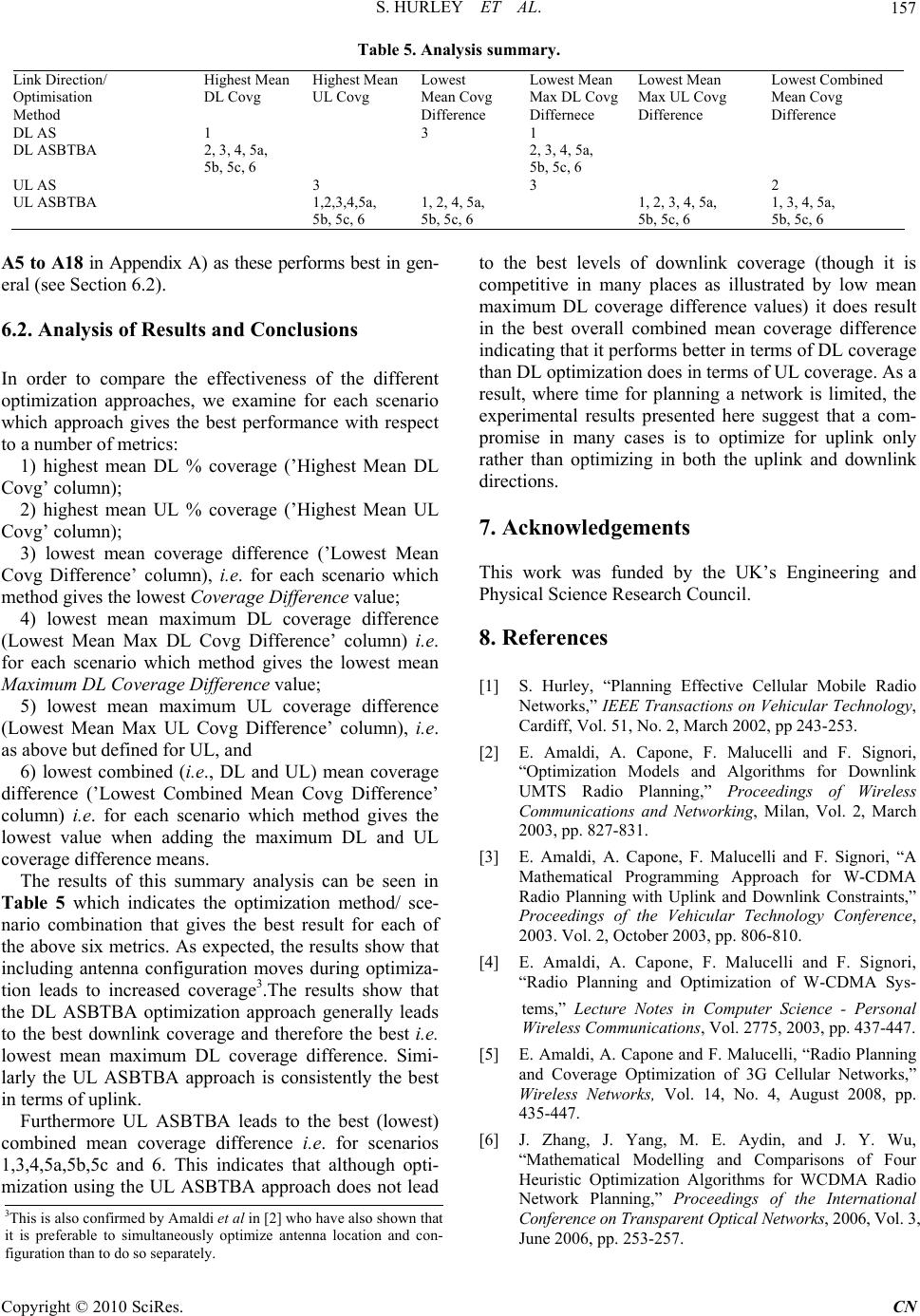

S. HURLEY ET AL.157
Table 5. Analysis summary.
Link Direction/
Optimisation
Highest Mean
DL Covg
Highest Mean
UL Covg
Lowest
Mean Covg
Lowest Mean
Max DL Covg
Lowest Mean
Max UL Covg
Lowest Combined
Mean Covg
Method Difference Differnece Difference Difference
DL AS 1 3 1
DL ASBTBA 2, 3, 4, 5a, 2, 3, 4, 5a,
5b, 5c, 6 5b, 5c, 6
UL AS 3 3 2
UL ASBTBA 1,2,3,4,5a, 1, 2, 4, 5a, 1, 2, 3, 4, 5a, 1, 3, 4, 5a,
5b, 5c, 6 5b, 5c, 6 5b, 5c, 6 5b, 5c, 6
A5 to A18 in Appendix A) as these performs best in gen-
eral (see Section 6.2).
6.2. Analysis of Results and Conclusions
In order to compare the effectiveness of the different
optimization approaches, we examine for each scenario
which approach gives the best performance with respect
to a number of metrics:
1) highest mean DL % coverage (’Highest Mean DL
Covg’ column);
2) highest mean UL % coverage (’Highest Mean UL
Covg’ column);
3) lowest mean coverage difference (’Lowest Mean
Covg Difference’ column), i.e. for each scenario which
method gives the lowest Coverage Difference value;
4) lowest mean maximum DL coverage difference
(Lowest Mean Max DL Covg Difference’ column) i.e.
for each scenario which method gives the lowest mean
Maximum DL Coverage Difference value;
5) lowest mean maximum UL coverage difference
(Lowest Mean Max UL Covg Difference’ column), i.e.
as above but defined for UL, and
6) lowest combined (i.e., DL and UL) mean coverage
difference (’Lowest Combined Mean Covg Difference’
column) i.e. for each scenario which method gives the
lowest value when adding the maximum DL and UL
coverage difference means.
The results of this summary analysis can be seen in
Table 5 which indicates the optimization method/ sce-
nario combination that gives the best result for each of
the above six metrics. As expected, the results show that
including antenna configuration moves during optimiza-
tion leads to increased coverage3.The results show that
the DL ASBTBA optimization approach generally leads
to the best downlink coverage and therefore the best i.e.
lowest mean maximum DL coverage difference. Simi-
larly the UL ASBTBA approach is consistently the best
in terms of uplink.
Furthermore UL ASBTBA leads to the best (lowest)
combined mean coverage difference i.e. for scenarios
1,3,4,5a,5b,5c and 6. This indicates that although opti-
mization using the UL ASBTBA approach does not lead
to the best levels of downlink coverage (though it is
competitive in many places as illustrated by low mean
maximum DL coverage difference values) it does result
in the best overall combined mean coverage difference
indicating that it performs better in terms of DL coverage
than DL optimization does in terms of UL coverage. As a
result, where time for planning a network is limited, the
experimental results presented here suggest that a com-
promise in many cases is to optimize for uplink only
rather than optimizing in both the uplink and downlink
directions.
7. Acknowledgements
This work was funded by the UK’s Engineering and
Physical Science Research Council.
8. References
[1] S. Hurley, “Planning Effective Cellular Mobile Radio
Networks,” IEEE Transactions on Vehicular Technology,
Cardiff, Vol. 51, No. 2, March 2002, pp 243-253.
[2] E. Amaldi, A. Capone, F. Malucelli and F. Signori,
“Optimization Models and Algorithms for Downlink
UMTS Radio Planning,” Proceedings of Wireless
Communications and Networking, Milan, Vol. 2, March
2003, pp. 827-831.
[3] E. Amaldi, A. Capone, F. Malucelli and F. Signori, “A
Mathematical Programming Approach for W-CDMA
Radio Planning with Uplink and Downlink Constraints,”
Proceedings of the Vehicular Technology Conference,
2003. Vol. 2, October 2003, pp. 806-810.
[4] E. Amaldi, A. Capone, F. Malucelli and F. Signori,
“Radio Planning and Optimization of W-CDMA Sys-
tems,” Lecture Notes in Computer Science - Personal
Wireless Communications, Vol. 2775, 2003, pp. 437-447.
[5] E. Amaldi, A. Capone and F. Malucelli, “Radio Planning
and Coverage Optimization of 3G Cellular Networks,”
Wireless Networks, Vol. 14, No. 4, August 2008, pp.
435-447.
[6] J. Zhang, J. Yang, M. E. Aydin, and J. Y. Wu,
“Mathematical Modelling and Comparisons of Four
Heuristic Optimization Algorithms for WCDMA Radio
Network Planning,” Proceedings of the International
Conference on Transparent Optical Networks, 2006, Vol. 3,
June 2006, pp. 253-257.
3This is also confirmed by Amaldi et al in [2] who have also shown tha
t
it is preferable to simultaneously optimize antenna location and con-
figuration than to do so separately.

S. HURLEY ET AL. 158
[7] J. Yang, M. E. Aydin, J. Zhang and C. Maple, “UMTS
Base Station Location Planning: a Mathematical Model
and Heuristic Optimisation Algorithms,”Communications,
Vol. 1, No. 5, October 2007, pp. 1007-1014.
[8] S. B. Jamaa, Z. Altman, J. M. Picard and B. Fourestie,
“Multi-objective Strategies for Automatic Cell Planning
of UMTS Networks,” Proceedings of the Vehicular
Technology Conference, Vol. 4, May 2004, pp. 2420-2424.
[9] S. B. Jamaa, Z. Altman, J. M. Picard and B. Fourestie,
“Combined Coverage and Capacity Optimisation for
UMTS Networks,” Telecommunications Network Strategy
and Planning Symposium, Moulineaux June 2004, pp.
175-178.
[10] R. M. Whitaker, S. Allen and S. Hurley, “Efficient
Offline Coverage and Load Evaluation for CDMA
Network Modeling,” IEEE Transactions on Vehicular
Technology, Vol. 58, No. 7, August 2009, pp 3704-3712.
[11] L. Mendo and J. M. Hernando, “On Dimension Reduc-
tion for Next Generation Microcellular Networks,” IEEE
Transactions of Communications, Vol. 49, No. 2, 2001,
pp. 243-248
[12] F. W. Glover and M. Laguna, “Tabu Search,” Springer,
1997.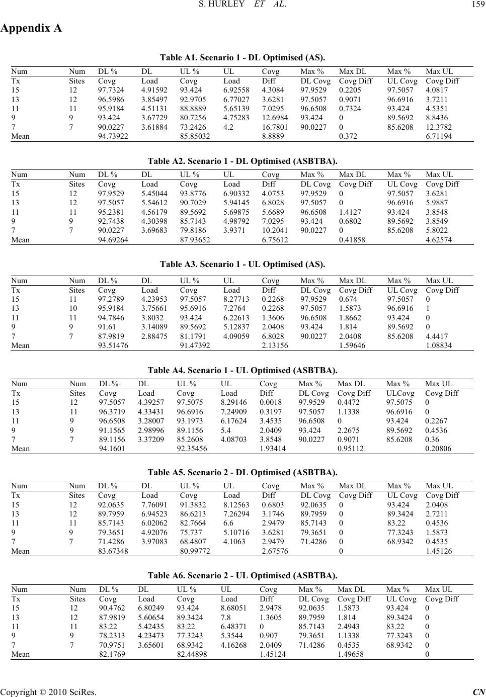

S. HURLEY ET AL.159
Appendix A
Table A1. Scenario 1 - DL Optimised (AS).
Num Num DL % DL UL % UL Covg Max % Max DL Max % Max UL
Tx Sites Covg Load Covg Load Diff DL Covg Covg Diff UL Covg Covg Diff
15 12 97.7324 4.91592 93.424 6.92558 4.3084 97.9529 0.2205 97.5057 4.0817
13 12 96.5986 3.85497 92.9705 6.77027 3.6281 97.5057 0.9071 96.6916 3.7211
11 11 95.9184 4.51131 88.8889 5.65139 7.0295 96.6508 0.7324 93.424 4.5351
9 9 93.424 3.67729 80.7256 4.75283 12.6984 93.424 0 89.5692 8.8436
7 7 90.0227 3.61884 73.2426 4.2 16.7801 90.0227 0 85.6208 12.3782
Mean 94.73922 85.85032 8.8889 0.372 6.71194
Table A2. Scenario 1 - DL Optimised (ASBTBA).
Num Num DL % DL UL % UL Covg Max % Max DL Max % Max UL
Tx Sites Covg Load Covg Load Diff DL Covg Covg Diff UL Covg Covg Diff
15 12 97.9529 5.45044 93.8776 6.90332 4.0753 97.9529 0 97.5057 3.6281
13 12 97.5057 5.54612 90.7029 5.94145 6.8028 97.5057 0 96.6916 5.9887
11 11 95.2381 4.56179 89.5692 5.69875 5.6689 96.6508 1.4127 93.424 3.8548
9 9 92.7438 4.30398 85.7143 4.98792 7.0295 93.424 0.6802 89.5692 3.8549
7 7 90.0227 3.69683 79.8186 3.9371 10.2041 90.0227 0 85.6208 5.8022
Mean 94.69264 87.93652 6.75612 0.41858 4.62574
Table A3. Scenario 1 - UL Optimised (AS).
Num Num DL % DL UL % UL Covg Max % Max DL Max % Max UL
Tx Sites Covg Load Covg Load Diff DL Covg Covg Diff UL Covg Covg Diff
15 11 97.2789 4.23953 97.5057 8.27713 0.2268 97.9529 0.674 97.5057 0
13 10 95.9184 3.75661 95.6916 7.2764 0.2268 97.5057 1.5873 96.6916 1
11 11 94.7846 3.8032 93.424 6.22613 1.3606 96.6508 1.8662 93.424 0
9 9 91.61 3.14089 89.5692 5.12837 2.0408 93.424 1.814 89.5692 0
7 7 87.9819 2.88475 81.1791 4.09059 6.8028 90.0227 2.0408 85.6208 4.4417
Mean 93.51476 91.47392 2.13156 1.59646 1.08834
Table A4. Scenario 1 - UL Optimised (ASBTBA).
Num Num DL % DL UL % UL Covg Max % Max DL Max % Max UL
Tx Sites Covg Load Covg Load Diff DL Covg Covg Diff ULCovg Covg Diff
15 12 97.5057 4.39257 97.5075 8.29146 0.0018 97.9529 0.4472 97.5075 0
13 11 96.3719 4.33431 96.6916 7.24909 0.3197 97.5057 1.1338 96.6916 0
11 9 96.6508 3.28007 93.1973 6.17624 3.4535 96.6508 0 93.424 0.2267
9 9 91.1565 2.98996 89.1156 5.4 2.0409 93.424 2.2675 89.5692 0.4536
7 7 89.1156 3.37209 85.2608 4.08703 3.8548 90.0227 0.9071 85.6208 0.36
Mean 94.1601 92.35456 1.93414 0.95112 0.20806
Table A5. Scenario 2 - DL Optimised (ASBTBA).
Num Num DL % DL UL % UL Covg Max % Max DL Max % Max UL
Tx Sites Covg Load Covg Load Diff DL Covg Covg Diff UL Covg Covg Diff
15 12 92.0635 7.76091 91.3832 8.12563 0.6803 92.0635 0 93.424 2.0408
13 12 89.7959 6.94523 86.6213 7.26294 3.1746 89.7959 0 89.3424 2.7211
11 11 85.7143 6.02062 82.7664 6.6 2.9479 85.7143 0 83.22 0.4536
9 9 79.3651 4.92076 75.737 5.10716 3.6281 79.3651 0 77.3243 1.5873
7 7 71.4286 3.97083 68.4807 4.1063 2.9479 71.4286 0 68.9342 0.4535
Mean 83.67348 80.99772 2.67576 0 1.45126
Table A6. Scenario 2 - UL Optimised (ASBTBA).
Num Num DL % DL UL % UL Covg Max % Max DL Max % Max UL
Tx Sites Covg Load Covg Load Diff DL Covg Covg Diff UL Covg Covg Diff
15 12 90.4762 6.80249 93.424 8.68051 2.9478 92.0635 1.5873 93.424 0
13 12 87.9819 5.60654 89.3424 7.8 1.3605 89.7959 1.814 89.3424 0
11 11 83.22 5.42435 83.22 6.48371 0 85.7143 2.4943 83.22 0
9 9 78.2313 4.23473 77.3243 5.3544 0.907 79.3651 1.1338 77.3243 0
7 7 70.9751 3.65601 68.9342 4.16268 2.0409 71.4286 0.4535 68.9342 0
Mean 82.1769 82.44898 1.45124 1.49658 0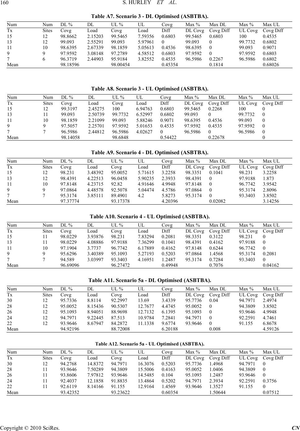

S. HURLEY ET AL. 160
Table A7. Scenario 3 - DL Optimised (ASBTBA).
Num Num DL % DL UL % UL Covg Max % Max DL Max % Max UL
Tx Sites Covg Load Covg Load Diff DL Covg Covg Diff UL Covg Covg Diff
15 12 98.8662 2.15203 99.5465 7.59356 0.6803 99.5465 0.6803 100 0.4535
13 12 99.093 2.55291 99.093 5.97961 0 99.093 0 99.7732 0.6802
11 10 98.6395 2.67339 98.1859 5.05613 0.4536 98.6395 0 99.093 0.9071
9 9 97.9592 3.08148 97.2789 4.58512 0.6803 97.9592 0 97.9592 0.6803
7 6 96.3719 2.44903 95.9184 3.82552 0.4535 96.5986 0.2267 96.5986 0.6802
Mean 98.18596 98.00454 0.45354 0.1814 0.68026
Table A8. Scenario 3 - UL Optimised (ASBTBA).
Num Num DL % DL UL % UL Covg Max % Max DL Max % Max UL
Tx Sites Covg Load Covg Load Diff DL Covg Covg Diff UL Covg Covg Diff
15 12 99.3197 2.45275 100 6.94763 0.6803 99.5465 0.2268 100 0
13 11 99.093 2.50739 99.7732 6.52997 0.6802 99.093 0 99.7732 0
11 10 98.1859 2.21099 99.093 5.88246 0.9071 98.6395 0.4536 99.093 0
9 9 97.5057 2.25701 97.9592 5.01653 0.4535 97.9592 0.4535 97.9592 0
7 7 96.5986 2.44812 96.5986 4.02627 0 96.5986 0 96.5986 0
Mean 98.14058 98.6848 0.54422 0.22678 0
Table A9. Scenario 4 - DL Optimised (ASBTBA).
Num Num DL % DL UL % UL Covg Max % Max DL Max % Max UL
Tx Sites Covg Load Covg Load Diff DL Covg Covg Diff UL Covg Covg Diff
15 12 98.231 3.48392 95.0052 5.71615 3.2258 98.3351 0.1041 98.231 3.2258
13 12 98.4391 4.22513 96.0458 5.90235 2.3933 98.4391 0 97.9188 1.873
11 10 97.8148 4.23715 92.82 4.91646 4.9948 97.8148 0 96.7742 3.9542
9 9 97.0864 4.48578 92.5078 5.04474 4.5786 97.0864 0 95.3174 2.8096
7 7 95.3174 3.85111 89.4901 4.2 5.8273 95.3174 0 93.3403 3.8502
Mean 97.37774 93.17378 4.20396 0.02082 3.14256
Table A10. Scenario 4 - UL Optimised (ASBTBA).
Num Num DL % DL UL % UL Covg Max % Max DL Max % Max UL
Tx Sites Covg Load Covg Load Diff DL Covg Covg Diff UL Covg Covg Diff
15 11 98.0229 3.93876 98.231 7.83294 0.2081 98.3351 0.3122 98.231 0
13 11 98.0229 4.08886 97.9188 7.36299 0.1041 98.4391 0.4162 97.9188 0
11 10 97.1904 3.7737 96.7742 6.17889 0.4162 97.8148 0.6244 96.7742 0
9 9 95.6296 3.40389 95.1093 5.27193 0.5203 97.0864 1.4568 95.3174 0.2081
7 7 94.589 3.03997 93.3403 4.16951 1.2487 95.3174 0.7284 93.3403 0
Mean 96.69096 96.27472 0.49948 0.7076 0.04162
Table A11. Scenario 5a - DL Optimised (ASBTBA).
Num Num DL % DL UL % UL Covg Max % Max DL Max % Max UL
Tx Sites Covg Load Covg Load Diff DL Covg Covg Diff UL Covg Covg Diff
30 12 95.7336 8.8114 92.2997 13.69 3.4339 95.7736 0.04 94.7971 2.4974
28 12 95.0052 8.15436 90.5307 12.7677 4.4745 95.0052 0 94.3809 3.8502
26 12 95.1093 8.94051 88.9698 12.7132 6.1395 95.1093 0 93.9646 4.9948
24 12 94.7971 9.22445 87.513 10.9784 7.2841 94.7971 0 92.2591 4.7461
22 12 93.9646 8.67947 84.2872 11.1338 9.6774 93.9646 0 91.155 6.8678
Mean 94.92196 88.72008 6.20188 0.008 4.59126
Table A12. Scenario 5a - UL Optimised (ASBTBA).
Num Num DL % DL UL % UL Covg Max % Max DL Max % Max UL
Tx Sites Covg Load Covg Load Diff DL Covg Covg Diff UL Covg Covg Diff
30 12 94.2768 14.8372 94.7971 16.3076 0.5203 95.7736 1.4968 94.7971 0
28 11 93.9646 7.50289 94.3809 15.5006 0.4163 95.0052 1.0406 94.3809 0
26 11 93.8606 7.97812 93.9646 14.5485 0.104 95.1093 1.2487 93.9646 0
24 11 92.4037 12.1858 91.8835 13.4864 0.5202 94.7971 2.3934 92.2591 0.3756
22 11 92.6119 8.14166 91.155 12.9164 1.4569 93.9646 1.3527 91.155 0
Mean 93.42352 93.23622 0.60354 1.50644 0.07512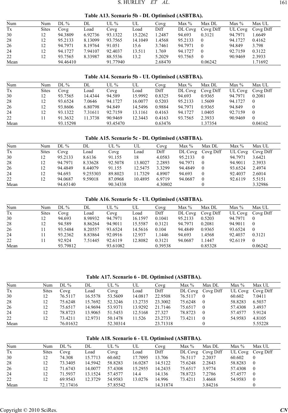

S. HURLEY ET AL. 161
Table A13. Scenario 5b - DL Optimised (ASBTBA).
Num Num DL % DL UL % UL Covg Max % Max DL Max % Max UL
Tx Sites Covg Load Covg Load Diff DL Covg Covg Diff UL Covg Covg Diff
30 12 94.3809 6.92736 93.1322 15.2262 1.2487 94.693 0.3121 94.7971 1.6649
28 12 95.2133 8.13099 93.7565 14.1049 1.4568 95.2133 0 94.1727 0.4162
26 12 94.7971 8.19764 91.051 15.6 3.7461 94.7971 0 94.849 3.798
24 12 94.1727 7.94107 92.4037 13.511 1.769 94.1727 0 92.7159 0.3122
22 12 93.7565 8.33987 88.5536 13.2 5.2029 93.7565 0 90.9469 2.3933
Mean 94.46410 91.77940 2.68470 0.06242 1.71692
Table A14. Scenario 5b - UL Optimised (ASBTBA).
Num Num DL % DL UL % UL Covg Max % Max DL Max % Max UL
Tx Sites Covg Load Covg Load Diff DL Covg Covg Diff UL Covg Covg Diff
30 12 93.7565 14.4344 94.589 15.9992 0.8325 94.693 0.9365 94.7971 0.2081
28 12 93.6524 7.0646 94.1727 16.0077 0.5203 95.2133 1.5609 94.1727 0
26 12 93.8606 6.80798 94.849 14.5496 0.9884 94.7971 0.9365 94.849 0
24 12 93.1322 7.31611 92.7159 13.1161 0.4163 94.1727 1.0405 92.7159 0
22 11 91.3632 11.3738 90.9469 12.3443 0.4163 93.7565 2.3933 90.9469 0
Mean 93.15298 93.45470 0.63476 1.37354 0.04162
Table A15. Scenario 5c - DL Optimised (ASBTBA).
Num Num DL % DL UL % UL Covg Max % Max DL Max % Max UL
Tx Sites Covg Load Covg Load Diff DL Covg Covg Diff UL Covg Covg Diff
30 12 95.2133 8.6136 91.155 18 4.0583 95.2133 0 94.7971 3.6421
28 12 94.7971 8.33628 92.5078 13.8027 2.2893 94.7971 0 94.9011 2.3933
26 12 94.4849 8.44079 91.155 12.5475 3.3299 94.4849 0 93.6524 2.4974
24 12 94.693 9.255303 89.8023 11.7329 4.8907 94.693 0 92.4037 2.6014
22 12 94.0687 9.59018 87.0968 10.4895 6.9719 94.0687 0 92.6119 5.5151
Mean 94.65140 90.34338 4.30802 0 3.32986
Table A16. Scenario 5c - UL Optimised (ASBTBA).
Num Num DL % DL UL % UL Covg Max % Max DL Max % Max UL
Tx Sites Covg Load Covg Load Diff DL Covg Covg Diff UL Covg Covg Diff
30 12 94.693 8.98932 94.7971 16.1597 0.1041 95.2133 0.5203 94.7971 0
28 12 94.589 8.86264 94.9011 15.5587 0.3121 94.7971 0.2081 94.9011 0
26 11 93.5484 8.20557 93.6524 14.5616 0.104 94.4849 0.9365 93.6524 0
24 11 93.2362 8.83864 92.0916 12.937 1.1446 94.693 1.4568 92.4037 0.3121
22 11 92.924 7.51445 92.6119 12.8082 0.3121 94.0687 1.1447 92.6119 0
Mean 93.79812 93.61082 0.39538 0.85328 0.06242
Table A17. Scenario 6 - DL Optimised (ASBTBA).
Num Num DL % DL UL % UL Covg Max % Max DL Max % Max UL
Tx Sites Covg Load Covg Load Diff DL CovgCovg Diff UL Covg Covg Diff
30 12 76.5117 16.5578 53.5609 14.0817 22.9508 76.5117 0 60.602 7.0411
28 12 75.6248 15.7692 52.3246 13.2735 23.3002 75.6248 0 58.8283 6.5037
26 12 75.6517 14.9694 53.9371 13.9292 21.7146 75.6517 0 57.4308 3.4937
24 12 78.8723 13.9065 51.5453 12.5168 27.327 78.8723 0 57.4577 5.9124
22 12 73.4211 12.9731 50.1478 11.526 23.2733 73.4211 0 54.9583 4.8105
Mean 76.01632 52.30314 23.71318 0 5.55228
Table A18. Scenario 6 - UL Optimised (ASBTBA).
Num Num DL % DL UL % UL Covg Max % Max DL Max % Max UL
Tx Sites Covg Load Covg Load Diff DL CovgCovg Diff UL Covg Covg Diff
30 12 74.308 15.7713 60.602 17.7095 13.706 76.5117 2.2037 60.602 0
28 12 73.3405 14.5942 58.8283 16.0287 14.5122 75.6248 2.2843 58.8283 0
26 12 71.6743 14.0077 57.4308 15.2955 14.2435 75.6517 3.9774 57.4308 0
24 12 71.5937 13.1524 57.4577 14.4 14.136 78.8723 7.2786 57.4577 0
22 12 69.9543 12.3729 54.9583 13.0276 14.996 73.4211 3.4668 54.9583 0
Mean 72.17416 57.85542 14.31874 3.84216 0