Journal of Global Positioning Systems (2004)
Vol. 3, No. 1-2: 115-131
An analysis of the effects of different network-based ionosphere
estimation models on rover positioning accuracy
Dorota A. Grejner-Brzezinska1, Pawel Wielgosz1,2, Israel Kashani1,3, Dru A. Smith4, Paul S. J. Spencer4,
Douglas S. Robertson4 and Gerald L. Mader4
1 The Ohio State University, SPIN LAB, 470 Hitchcock Hall, 2070 Neil Ave., Columbus, OH 43210-1275
e-mail: [e-mail]; Tel: [phone]; Fax: [phone]
2 University of Warmia and Mazury – UWM
3 Israel Institute of Technology – Technion
4 National Geodetic Survey – NGS
Received: 15 Nov 2004 / Accepted: 3 Feb 2005
Abstract. The primary objective of this paper is to test
several methods of modeling the ionospheric corrections
derived from a reference GPS network, and to study the
impact of the models’ accuracy on the user positioning
results. The five ionospheric models that are discussed
here are: (1) network RTK (NR) carrier phase-based
model — MPGPS-NR, (2) absolute, smoothed
pseudorange-based model — MPGPS-P4, (3) IGS Global
Ionosphere Model — GIM, (4) absolute model based on
undifferenced dual-frequency ambiguous carrier phase
data — ICON, and (5) carrier phase-based data
assimilation method — MAGIC. Methods 1–4 assume
that the ionosphere is an infinitesimal single layer, while
method (5) considers the ionosphere as a 3D medium.The
test data set was collected at the Ohio Continuously
Operating Reference Stations (CORS) network on August
31, 2003. A 24-hour data set, representing moderate
ionospheric conditions (maximum Kp = 2o), was
processed. The ionospheric reference “truth” in double-
difference (DD) form was generated from the dual-
frequency carrier phase data for two selected baselines,
~60 and ~100 km long, where one station was considered
as a user receiver at an unknown location (simulated
rover). The five ionospheric models were used to
generate the DD ionospheric corrections for the rover,
and were compared to the reference “truth.” The quality
statistics were generated and discussed. Examples of
instantaneous ambiguity resolution and RTK positioning
are presented, together with the accuracy requirements
for the ionospheric corrections, to assure integer
ambiguity fixing.
Key words: Network-based RTK, ionospheric models,
ambiguity resolution.
1 Introduction
One of the major limiting factors in GPS-based precise
positioning is the ionosphere-induced propagation delay
that, if not properly accounted for, may result in
significant positioning errors. This is particularly true for
single frequency data, reducing the length of the effective
baseline to 10–15 km. While dual-frequency carrier phase
measurements can form an ionosphere-free linear
combination that removes first-order ionospheric errors,
the integer ambiguities can be fixed only for short
baselines, since the ionospheric error decorrelates with
distance. The ionospheric signal delay is a function of the
total electron content (TEC). TEC is defined as the total
number of electrons contained in a column with a cross-
sectional area of 1 m2 along the signal path. TEC displays
primarily day-to-night variations, but also depends on the
geomagnetic latitude, time of year, and the sunspot cycle.
It is measured in electron/m2, where one total electron
content unit (TECU) is defined as 1016 electron/m2. One
meter of the ionospheric delay (or advance) on the first
GPS frequency corresponds to 6.16 TECU, or one TECU
causes 0.162 m delay.
The ability to remove the ionospheric delay from GPS
data can increase the performance of the integer

116 Journal of Global Positioning Systems
ambiguity resolution (AR) process, and improve the
computational efficiency of the search process. However,
due to the high-level variability of TEC, empirical
ionospheric models do not provide sufficient accuracy to
support high-precision positioning applications. On the
other hand, if external information on the integrated TEC
between pairs of satellites and receivers is provided based
on real observation data, the base-rover separation can be
significantly extended, resulting in a virtually “distance-
independent” precise positioning. The external
ionospheric information provides an important constraint
for accurate and rapid carrier phase AR. An alternative
approach is to estimate the double-difference (DD)
ionospheric delay parameters in the positioning
adjustment model. However, the underlying mathematical
model becomes weaker, and as a consequence the
required observation sessions become longer (Odijk,
2000); thus, this method does not apply to rapid static or
kinematic algorithms where the occupation time is of the
order of seconds to minutes.
Several methods have been proposed to estimate and
model the ionospheric corrections from the ground-based
GPS data from the Continuously Operating Reference
Stations (CORS) network, and the mathematical
representation of the ionospheric electron density field
have been studied (see, for example Odijk, 2000 and
2001; Schaer, 1999; Wielgosz et al., 2003; Kashani et al.,
2004a; Smith, 2004; Spencer et al., 2004) to support
network-based real-time kinematic (RTK) (see, for
example, Vollath et al., 2000; Rizos, 2002; Wanninger,
2002; Grejner-Brzezinska et al., 2004a and 2004b). The
most challenging among these methods is the
instantaneous AR approach (Kim and Langley, 2000),
where for each individual observation epoch a new
integer ambiguity solution is obtained using only the
current epoch data (Bock et al., 2003). Consequently, this
method is resistant to negative effects of cycle slips and
gaps, and can provide centimeter-level positioning
accuracy immediately, without any delay needed for
initialization (or re-initialization). However, to
successfully resolve the ambiguities instantaneously over
long distances, external atmospheric corrections of high
accuracy are required (Odijk, 2001; Kashani et al.,
2004b).
This paper presents the accuracy analysis of several
methods of ionospheric correction modeling in
comparison to reference “truth,” using the Multi Purpose
GPS Processing Software (MPGPS™) developed at the
Satellite Positioning and Inertial Navigation (SPIN)
group at The Ohio State University. The ionospheric
corrections are represented by the DD ionospheric delays
estimated directly from dual-frequency carrier phase data
constrained by the integer ambiguities. Examples of the
positioning accuracy, supported by instantaneous AR,
achieved as a function of the ionospheric correction
quality are also presented and discussed. The five
ionospheric models tested are listed below.
MPGPS-NR — Network RTK (NR) carrier phase-based
model, decomposed from DD ionospheric delays
(Kashani et al., 2004a),
MPGPS-P4 — Absolute, smoothed pseudorange-based
method (Wielgosz et al., 2003),
IGS GIM — International GPS Service (IGS) global
ionospheric map (GIM). IGS GIM is a combination of
several different ionosphere models provided by the IGS
Ionosphere Associate Analysis Centers (Schaer, 1999),
ICON — Absolute model based on undifferenced dual-
frequency ambiguous carrier phase data (Smith, 2004),
MAGIC — Pseudorange-leveled carrier phase-based data
assimilation method (Spencer et al., 2004).
Methods 1–4 assume that the ionosphere is an
infinitesimal single layer, while method 5 considers the
ionosphere as a 3D medium. In terms of spatial coverage,
methods 1 and 2 are considered local; methods 4 and 5
are regional, while method 3 offers global coverage.
MAGIC and ICON (4 and 5) are the two NGS ionosphere
models derived for the continental United States. These
two models use CORS GPS data, and provide the
ionospheric corrections with a three-day delay. Both
models are prototypes, a part of ongoing research
projects, and are currently available to the general public
for testing and evaluation purposes
(http://www.noaanews.noaa.gov/stories2004/s2333.htm).
2 Approach and methodology
This section provides a brief description of the algorithms
and methods applied to the aforementioned ionosphere
estimation models. In addition, the AR and rover
positioning algorithms are also briefly discussed. More
details can be found in the references provided in each
section.
2.1 The ionospheric models
2.1.1 The reference “truth” model — MPGPS-L4
The fundamental mathematical model for the network-
based adjustment, using dual-frequency carrier phase and
pseudorange data from the reference stations, is described
by Eq. (1). The system of equations (1) written for the
entire network is solved for each epoch of observations
using a generalization-based sequential least-squares
adjustment with stochastic constraints (Kashani et al.,
2004a).

Grejner-Brzezinska et al.: An analysis of the effects of different network-based ionosphere estimation models 117
1, 11,
22
2,122 2,
1,
2,
()0
()(/)0
()0
(
kl klklklklkl
ijiji iiijjjjijij
kl klklklklkl
ijiji iiij jjjijij
kl kl klklkl
ijijii iijjjjij
kl klklk
ijijiii ij
TT TTIN
TTT TIN
PTTTTI
PTT
Φρααααλ
Φρααα αυυλ
ρα ααα
ρααα
−−− −++−=
−−−−++−=
−−− −+−=
−−− −22
12
)( / )0
lkl
jjj ij
TT I αυυ +− =
(1)
where:
,ij receiver indices,
,kl satellite indices,
,
kl
nij
Φ DD phase observation on frequency n
(n=1,2),
,
kl
nij
P DD code observation on frequency n,
kl
ij
ρ
DD geometric distance,
,ij
T tropospheric total zenith delay (TZD),
k
i
α
troposphere mapping function,
kl
ij
I
DD ionospheric delay,
12
,
υ
υ L1 and L2 frequencies,
12
,
λ
λ GPS frequency wavelengths on L1 and L2,
1, 2,
,
kl kl
ij ij
NN DD carrier phase ambiguities on L1 and L2.
The unknown parameters are undifferenced total zenith
delay (TZD), provided for individual stations (,ij T), DD
ionospheric delays (kl
ij
I
), and DD ambiguities
(1, 2, ,
kl kl
ij ij
NN). The coordinates of the permanent stations
(CORS) are considered known (obtained from a 24-hour
solution using the BERNESE software (Hugentobler et
al., 2001)), which makes the AR for the reference
network much easier to perform, even for long-range
distances (i.e., ∼200 km between the CORS stations). All
the parameters are constrained to some a priori
information, which may consist of empirical values (e.g.,
30–50 cm for the DD ionospheric delays, depending on
the baseline length, local time and satellite elevation
angle), as well as variance-covariance matrix for the
known CORS coordinates. The Least-squares AMBiguity
Decorrelation Adjustment (LAMBDA) is used to fix the
ambiguities to their integer values (Teunissen, 1994). The
validation procedure used is the AR success rate
(Teunissen et al., 2002), which represents the probability
of estimating the correct integers.
After the DD ambiguities associated with the reference
receivers have been fixed to their correct integer values,
the “true” DD ionospheric delay can be correctly
estimated using the geometry-free linear combination
described by Eq. (2):
,441 1,22,
()0
kl klklkl
ijijijij
LI NN ξλλ
+
−− = (2)
where:
,4,1,2
klkl kl
ijij ij
LLL=−and
2
1
42
2
10.647
υ
ξυ
=− ≈−
It can be seen from Eq. (2) that if the dual-frequency
ambiguity parameters 1,
kl
ij
N and 2,
kl
ij
N are fixed to their
integers, the only remaining unknown parameter, kl
ij
I
,
representing the DD ionospheric delay on L1, can be
estimated with a few-millimeter accuracy, corresponding
primarily to the noise on the DD carrier phase
observables.
2.1.2 The carrier phase DD model — MPGPS-NR
The network-based approach presented is Section 2.1.1
was also used to derive the network-based ionospheric
corrections (MPGPS-NR). In this model, the zero
difference (ZD) ionospheric delays (i.e., one-way, biased)
were obtained by decomposing the network-derived DD
delays, and interpolated for the rover location (KNTN).
This was done for all satellites/epochs used in the
analyses presented in Section 3. The network solution did
not include the selected rover observations. It should be
mentioned that for an individual baseline and n DD
delays the rigorous decomposition is not possible without
the a priori knowledge of at least two ZD values; there
are only n-2 linearly independent DD observation
equations, thus the system is undetermined. To regularize
the normal matrix, independent constraints on at least two
ZD delays are needed, or loose constraints can be
introduced to the diagonal of the normal matrix. Both
methods result in a biased estimate. Although the
reconstruction of the DD delays from the interpolated ZD
delays may still include some amount of residual biases,
the resulting DD delays are generally of sufficient
accuracy to enable fast AR with only a few epochs of
data (see Kashani et al., 2004a).

118 Journal of Global Positioning Systems
2.1.3 The smoothed pseudorange model — MPGPS-
P4
In this approach (Wielgosz et al., 2003) dual-frequency
GPS carrier phase data are used to smooth the
pseudorange observations collected at the reference
station network (Springer, 1999). After the smoothing
procedure, the pseudoranges are effectively replaced by
the carrier phase observations with approximated (real-
value) ambiguities. The differential code biases (DCBs)
for the satellites are provided by IGS
(ftp://gage.upc.es/pub/gps_data/GPS_IONO), and for the
receivers, are derived from the calibration performed with
the BERNESE software (Hugentobler et al., 2001). The
instantaneous absolute ionospheric delay k
i
I
is computed
from Eq. (3):
,4 4
(( ))/
kk k
ii i
IPcbb ∆∆ξ =− +
 (3)
where:
i, j, k, l indices are the same as in Section 2.1.1,
,
k
in
P
 carrier-smoothed code observation on
frequency n (n=1,2),
,4
k
i
P
 geometry-free linear combination of smoothed
code observations ,4,1 ,2
kkk
iii
PPP=−

,
c speed of light,
k
b ∆ ,i b ∆ DCB for satellite k, and receiver i,
respectively,
4
ξ
coefficient converting ionospheric delay on P4 to
P1 delay (Eq. (2)).
The ionospheric delay is the following function of TEC
(Schaer, 1999):
2
1
2
kx
iTEC
C
I
TEC TEC υξ
−
=±= (4)
where the proportionality factor 2
x
C = 40.3 ×1016
ms-2/TECU, and the ionospheric delay caused by 1 TECU
on L1 is TEC
ξ
= 0.162 m/TECU.
2.1.4 The IGS GIM
The IGS GIMs are derived as a weighted combination of
several different models developed independently by the
IGS Ionosphere Associate Analysis Centers. The
combined maps have a spatial resolution of 2.5º and 5.0º
in latitude and longitude, respectively, and a 2-hour
temporal resolution (Feltens and Jakowski, 2002). IGS
GIMs assume a single layer model with the layer height,
H, at 450 km. To convert the vertical TEC (VTEC) from
GIMs into the line-of-sight slant TEC, a modified single-
layer model (MSLM) mapping function is adopted (Eq.
5).
1
() cos( ') FZ z =
with:
sin(')sin()
R
zz
RH
α
=+
/cos( ')TEC VTECz
=
(5)
where: F(z) is the mapping function, R is the Earth’s
radius, z is the vertical angle to the satellite, z´ is the
angle between the topocentric direction to the satellite
and the normal to the ionospheric layer through the pierce
point (piercing angle), and
α
is a scaling factor. GIMs
provide absolute TEC in the IONEX format (Schaer et
al., 1998). In this study, the ionospheric delays were
interpolated for the rover and base receiver locations
using kriging; they can subsequently be used to form DD
corrections in the rover-positioning step.
2.1.5 The carrier phase absolute model — ICON
This method of computing absolute (unambiguous) levels
of TEC (and subsequently L1 and L2 delays) from a
ground-based network of GPS receivers requires dual-
frequency carrier phase data. The ionosphere is assumed
to lie in a single layer of constant ellipsoidal height of
300 km, and the geographic locations of the GPS ground
stations must allow simultaneous observation of satellites
by a number of stations. Slant TEC derived from GPS
measurements is converted to VTEC, as shown in Eq. (5).
Considering dual-frequency data, one can derive Eq. (6)
to estimate the TEC difference between consecutive
epochs m and n, where κ corresponds to /2
x
C in Eq. (4).
Using Eq. (5), the TEC difference can be further
converted to the difference in VTEC, as shown in Eq. (7),
which represents the ambiguous VTEC as a function of
the unknown absolute TEC at epoch m. In these formulas,
ϕ
1 and
ϕ
2 are the carrier phase data in cycles.
()
,
1
,,
12
22
12
111
mnm n
mn mn
TECTEC TEC ∆
∆ϕ ∆ϕ
κυ υ
−
=−=

 −−




(6)
,
,
cos( ')cos( ')
cos( ')(cos( ')cos( '))
mnn m
nn mm
mn nmnm
VTECVTEC VTEC
TECz TECz
TECzTECzz
∆
∆
=−=
−=
+−
(7)

Grejner-Brzezinska et al.: An analysis of the effects of different network-based ionosphere estimation models 119
In order to estimate the bias (as only TEC time-difference
can be obtained from (6) or (7)), a concept of track
crossover is introduced, which is the fundamental notion of
this method. The term crossover is related here to any two
satellite tracks formed by the ionosphere pierce points,
that fall within some acceptably small tolerance (in both
space and time) of one another. Considering three tracks
forming a triangle, as shown in Figure 1, each of the three
tracks has one unknown bias (b1, b2 and b3),
corresponding to the absolute TEC value at some initial
epoch. If these biases were known, the absolute values of
TEC and VTEC at every epoch can be computed using
the biases and ∆VTEC defined in Eq. (7). Each crossover
A, B and C in Figure 1 forms a unique constraint for the
system (Eq. 8), which allows for absolute estimation of
VTEC. Adjoining “triangles,” shown in Figure 1, provide
more constraints introducing redundancy to the system.
For more details on this method, see (Smith, 2004). In
this study, the ionospheric delay values were computed
for entire continental U.S., using around 340 stations;
normally, for stations not included in the computations,
TEC (and delays) can be interpolated for the
station/satellite pair.
13
AAA
VTEC VTECVTEC==
12
B
BB
VTEC VTEC VTEC==
23
CCC
VTEC VTEC VTEC==
(8)
2.1.6 The carrier phase tomographic model —
MAGIC
A method used here to reconstruct the 3D Earth
ionospheric electron density field using a land-based
network of GPS receivers is referred to as the data
assimilation method. It uses a Kalman filter and can
combine data from various sources to obtain inversions in
three dimensions (Spencer et al., 2004). The primary
problem of the data assimilation method, which requires
some form of mathematical regularization, transpires
from the fact that the method is essentially a very poorly
constrained linear least squares problem. Continuity
relationships, defining the smoothness or entropy of the
solution, are often used regularization techniques in
tomographic methods (2D and 3D), while in cases of data
assimilation methods, an a priori model estimate of the
solution along with an estimate of its covariance are used.
MAGIC uses an optional mapping function to alter the
representation of the Kalman filter state vector in terms of
a set of discrete radial empirical orthonormal functions
(EOFs) to enable a more concise representation of the
state vector (the ionospheric electron density field) in
three dimensions (Spencer et al., 2004). The EOFs were
formed by applying singular value decomposition to a set
of model profiles generated by IRI95 (International
Reference Ionosphere; see, for example, Bilitza, 1997).
The dominant term, EOF1, represents a mean ionospheric
profile. Examples of empirical orthonormal functions are
illustrated in Figure 2.
The carrier phase geometry-free linear combination (L4)
leveled to the pseudorange is used as the GPS observable.
The solutions are quantized with 15-minute time-steps. In
this study, about 150 CORS and IGS stations were used
for the TEC (converted to ionospheric delay) estimation
for the continental US. For more details on this method,
see (Spencer et al., 2004).
2.2 The kinematic positioning algorithm
The concept of long-range instantaneous RTK GPS
presented here is based on the atmospheric corrections
derived from the GPS observations collected by the
reference network that supports the rover positioning.
The data reduction algorithm operates in the DD mode,
which requires receiving observations from at least one
reference station, together with the atmospheric
corrections, i.e., tropospheric, kl
ij
T, and ionospheric, kl
ij
I
,
as shown in Eq. 9.
1,1 1,
22
2,1222,
1,
22
2,1 2
0
(/) 0
0
(/)0
klklkl klkl
ijij ijijij
klkl klklkl
ij ijijijij
klklkl kl
ijij ijij
klkl klkl
ij ijijij
TI N
TffI N
PTI
PTffI
Φρ λ
Φρ λ
ρ
ρ
−
−+− =
−
−+−=
−
−− =
−
−− =
(9)
The fundamental observation equations for pseudorange
and carrier phase observations, parameterized according
to the generalization-based approach, are presented in Eq.
9, where the notation follows the previously explained
paradigm. Stochastic constraints are applied to the
atmospheric corrections and the LAMBDA method is
used for the AR. All the processing is carried out at the
rover receiver in the instantaneous mode. The success of
the instantaneous GPS positioning over long baselines
depends on the ability to resolve the integer phase
ambiguities. The performance of the method strongly
depends on the quality of the atmospheric corrections
provided from the network. If high quality corrections are
available, the method becomes virtually distance-
independent. The analyses presented in Section 3 are
aimed at estimating the required quality of these
corrections to assure seamless, instantaneous positioning
without any initialization, as required in the on-the-fly
(OTF) technique.
All the processing algorithms currently implemented in
the MPGPS™ software include the following modules:
long-range instantaneous and OTF RTK GPS, precise
point positioning (PPP), multi-station DGPS, ionosphere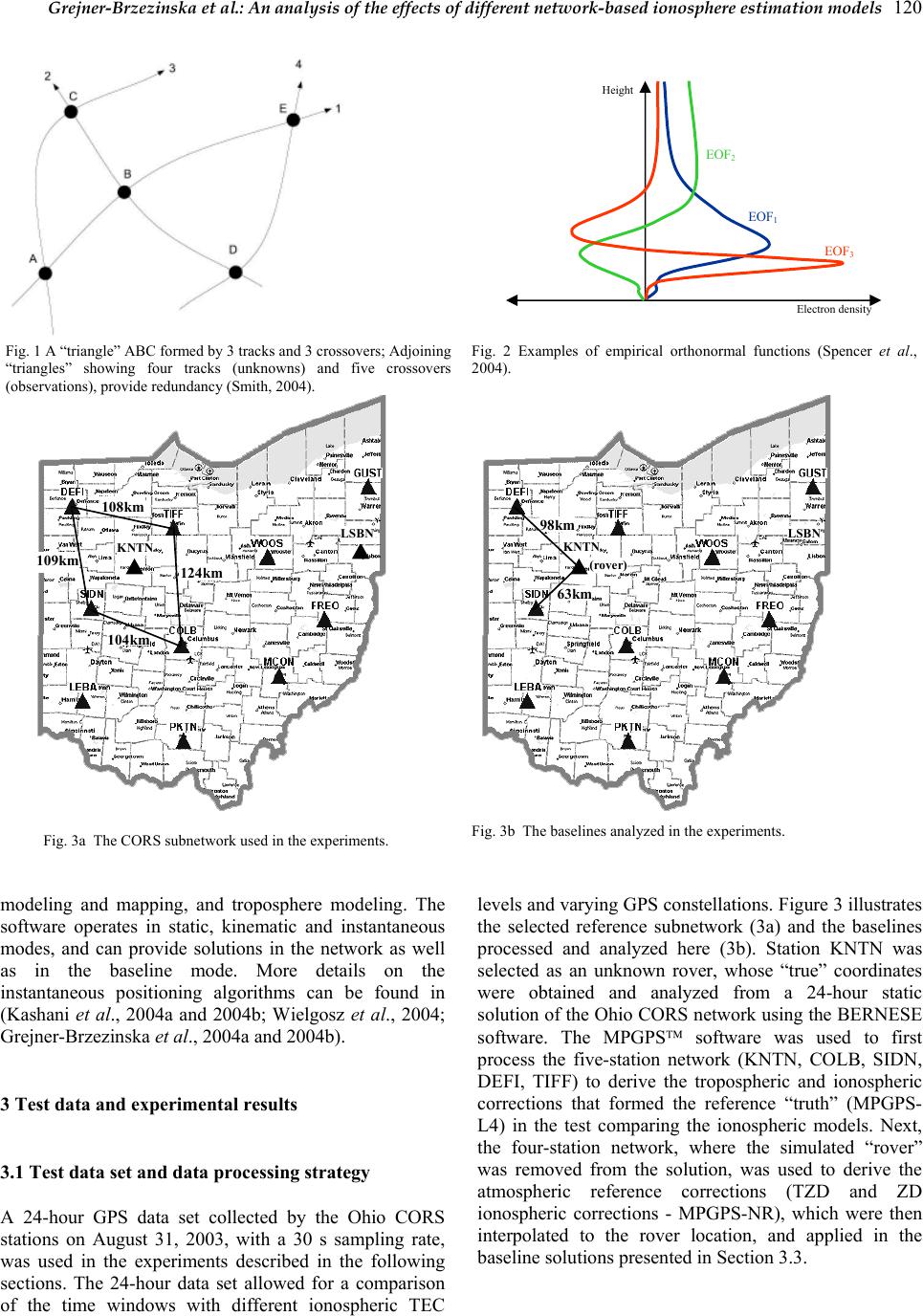

Grejner-Brzezinska et al.: An analysis of the effects of different network-based ionosphere estimation models 120
Fig. 1 A “triangle” ABC formed by 3 tracks and 3 crossovers; Adjoining
“triangles” showing four tracks (unknowns) and five crossovers
(observations), provide redundancy (Smith, 2004).
Fig. 2 Examples of empirical orthonormal functions (Spencer et al.,
2004).
104km
109km
124k m
108k m
KNTN
LSBN
63km
98km
KNTN
LSBN
(rover)
Fig. 3a The CORS subnetwork used in the experiments. Fig. 3b The baselines analyzed in the experiments.
modeling and mapping, and troposphere modeling. The
software operates in static, kinematic and instantaneous
modes, and can provide solutions in the network as well
as in the baseline mode. More details on the
instantaneous positioning algorithms can be found in
(Kashani et al., 2004a and 2004b; Wielgosz et al., 2004;
Grejner-Brzezinska et al., 2004a and 2004b).
3 Test data and experimental results
3.1 Test data set and data processing strategy
A 24-hour GPS data set collected by the Ohio CORS
stations on August 31, 2003, with a 30 s sampling rate,
was used in the experiments described in the following
sections. The 24-hour data set allowed for a comparison
of the time windows with different ionospheric TEC
levels and varying GPS constellations. Figure 3 illustrates
the selected reference subnetwork (3a) and the baselines
processed and analyzed here (3b). Station KNTN was
selected as an unknown rover, whose “true” coordinates
were obtained and analyzed from a 24-hour static
solution of the Ohio CORS network using the BERNESE
software. The MPGPS software was used to first
process the five-station network (KNTN, COLB, SIDN,
DEFI, TIFF) to derive the tropospheric and ionospheric
corrections that formed the reference “truth” (MPGPS-
L4) in the test comparing the ionospheric models. Next,
the four-station network, where the simulated “rover”
was removed from the solution, was used to derive the
atmospheric reference corrections (TZD and ZD
ionospheric corrections - MPGPS-NR), which were then
interpolated to the rover location, and applied in the
baseline solutions presented in Section 3.3.
Height
EOF1
EOF2
EOF3
Electron density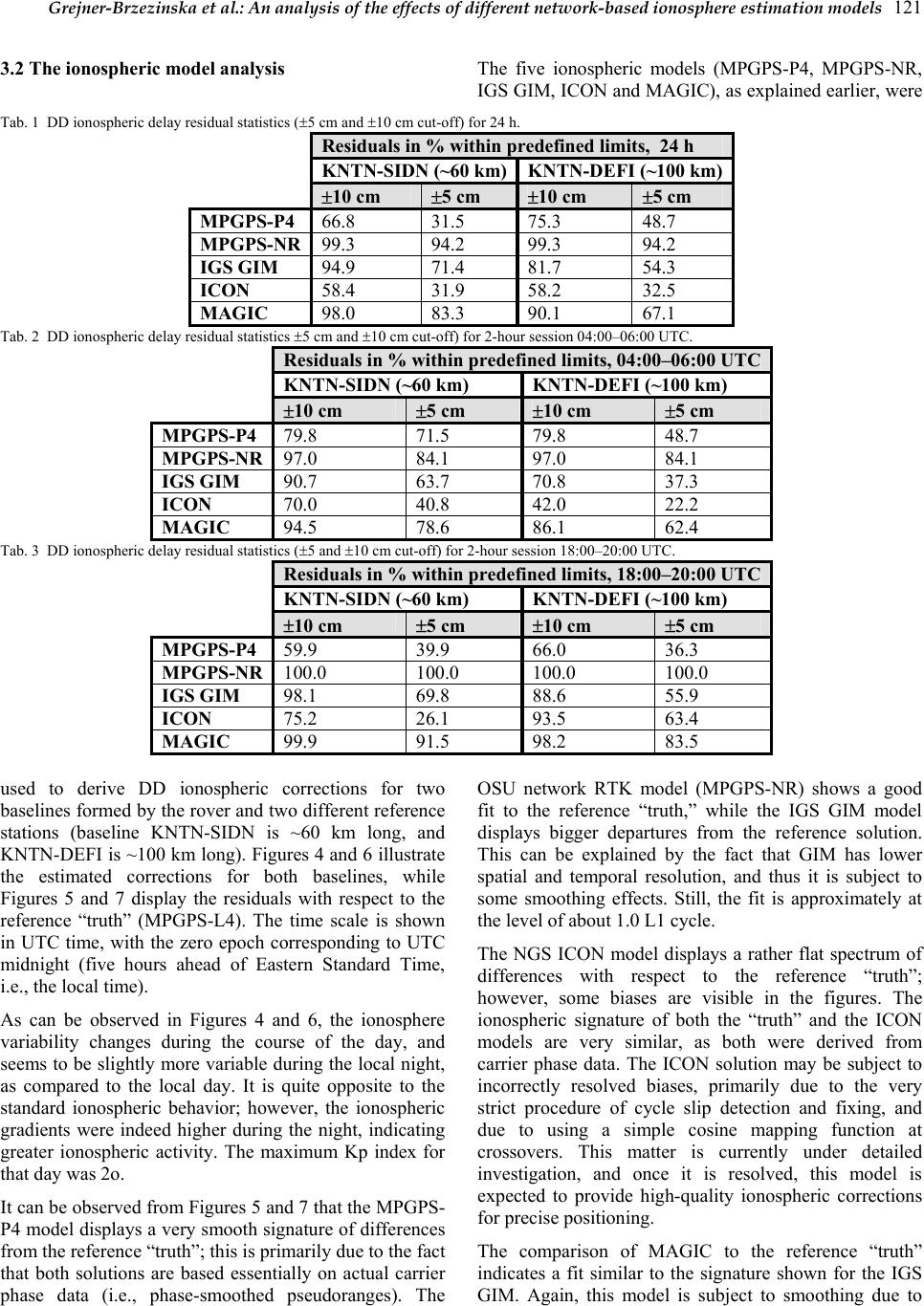

Grejner-Brzezinska et al.: An analysis of the effects of different network-based ionosphere estimation models 121
3.2 The ionospheric model analysis The five ionospheric models (MPGPS-P4, MPGPS-NR,
IGS GIM, ICON and MAGIC), as explained earlier, were
Tab. 1 DD ionospheric delay residual statistics (±5 cm and ±10 cm cut-off) for 24 h.
Residuals in % within predefined limits, 24 h
KNTN-SIDN (~60 km)KNTN-DEFI (~100 km)
±10 cm ±5 cm ±10 cm ±5 cm
MPGPS-P4 66.8 31.5 75.3 48.7
MPGPS-NR 99.3 94.2 99.3 94.2
IGS GIM 94.9 71.4 81.7 54.3
ICON 58.4 31.9 58.2 32.5
MAGIC 98.0 83.3 90.1 67.1
Tab. 2 DD ionospheric delay residual statistics ±5 cm and ±10 cm cut-off) for 2-hour session 04:00–06:00 UTC.
Residuals in % within predefined limits, 04:00–06:00 UTC
KNTN-SIDN (~60 km) KNTN-DEFI (~100 km)
±10 cm ±5 cm ±10 cm ±5 cm
MPGPS-P4 79.8 71.5 79.8 48.7
MPGPS-NR 97.0 84.1 97.0 84.1
IGS GIM 90.7 63.7 70.8 37.3
ICON 70.0 40.8 42.0 22.2
MAGIC 94.5 78.6 86.1 62.4
Tab. 3 DD ionospheric delay residual statistics (±5 and ±10 cm cut-off) for 2-hour session 18:00–20:00 UTC.
Residuals in % within predefined limits, 18:00–20:00 UTC
KNTN-SIDN (~60 km) KNTN-DEFI (~100 km)
±10 cm ±5 cm ±10 cm ±5 cm
MPGPS-P4 59.9 39.9 66.0 36.3
MPGPS-NR 100.0 100.0 100.0 100.0
IGS GIM 98.1 69.8 88.6 55.9
ICON 75.2 26.1 93.5 63.4
MAGIC 99.9 91.5 98.2 83.5
used to derive DD ionospheric corrections for two
baselines formed by the rover and two different reference
stations (baseline KNTN-SIDN is ~60 km long, and
KNTN-DEFI is ~100 km long). Figures 4 and 6 illustrate
the estimated corrections for both baselines, while
Figures 5 and 7 display the residuals with respect to the
reference “truth” (MPGPS-L4). The time scale is shown
in UTC time, with the zero epoch corresponding to UTC
midnight (five hours ahead of Eastern Standard Time,
i.e., the local time).
As can be observed in Figures 4 and 6, the ionosphere
variability changes during the course of the day, and
seems to be slightly more variable during the local night,
as compared to the local day. It is quite opposite to the
standard ionospheric behavior; however, the ionospheric
gradients were indeed higher during the night, indicating
greater ionospheric activity. The maximum Kp index for
that day was 2o.
It can be observed from Figures 5 and 7 that the MPGPS-
P4 model displays a very smooth signature of differences
from the reference “truth”; this is primarily due to the fact
that both solutions are based essentially on actual carrier
phase data (i.e., phase-smoothed pseudoranges). The
OSU network RTK model (MPGPS-NR) shows a good
fit to the reference “truth,” while the IGS GIM model
displays bigger departures from the reference solution.
This can be explained by the fact that GIM has lower
spatial and temporal resolution, and thus it is subject to
some smoothing effects. Still, the fit is approximately at
the level of about 1.0 L1 cycle.
The NGS ICON model displays a rather flat spectrum of
differences with respect to the reference “truth”;
however, some biases are visible in the figures. The
ionospheric signature of both the “truth” and the ICON
models are very similar, as both were derived from
carrier phase data. The ICON solution may be subject to
incorrectly resolved biases, primarily due to the very
strict procedure of cycle slip detection and fixing, and
due to using a simple cosine mapping function at
crossovers. This matter is currently under detailed
investigation, and once it is resolved, this model is
expected to provide high-quality ionospheric corrections
for precise positioning.
The comparison of MAGIC to the reference “truth”
indicates a fit similar to the signature shown for the IGS
GIM. Again, this model is subject to smoothing due to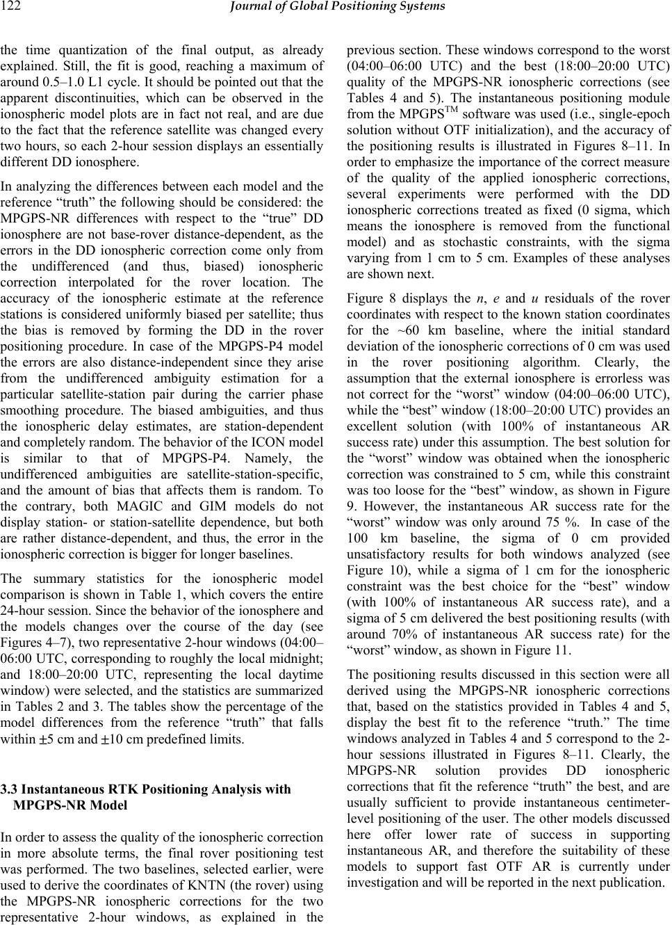

122 Journal of Global Positioning Systems
the time quantization of the final output, as already
explained. Still, the fit is good, reaching a maximum of
around 0.5–1.0 L1 cycle. It should be pointed out that the
apparent discontinuities, which can be observed in the
ionospheric model plots are in fact not real, and are due
to the fact that the reference satellite was changed every
two hours, so each 2-hour session displays an essentially
different DD ionosphere.
In analyzing the differences between each model and the
reference “truth” the following should be considered: the
MPGPS-NR differences with respect to the “true” DD
ionosphere are not base-rover distance-dependent, as the
errors in the DD ionospheric correction come only from
the undifferenced (and thus, biased) ionospheric
correction interpolated for the rover location. The
accuracy of the ionospheric estimate at the reference
stations is considered uniformly biased per satellite; thus
the bias is removed by forming the DD in the rover
positioning procedure. In case of the MPGPS-P4 model
the errors are also distance-independent since they arise
from the undifferenced ambiguity estimation for a
particular satellite-station pair during the carrier phase
smoothing procedure. The biased ambiguities, and thus
the ionospheric delay estimates, are station-dependent
and completely random. The behavior of the ICON model
is similar to that of MPGPS-P4. Namely, the
undifferenced ambiguities are satellite-station-specific,
and the amount of bias that affects them is random. To
the contrary, both MAGIC and GIM models do not
display station- or station-satellite dependence, but both
are rather distance-dependent, and thus, the error in the
ionospheric correction is bigger for longer baselines.
The summary statistics for the ionospheric model
comparison is shown in Table 1, which covers the entire
24-hour session. Since the behavior of the ionosphere and
the models changes over the course of the day (see
Figures 4–7), two representative 2-hour windows (04:00–
06:00 UTC, corresponding to roughly the local midnight;
and 18:00–20:00 UTC, representing the local daytime
window) were selected, and the statistics are summarized
in Tables 2 and 3. The tables show the percentage of the
model differences from the reference “truth” that falls
within ±5 cm and ±10 cm predefined limits.
3.3 Instantaneous RTK Positioning Analysis with
MPGPS-NR Model
In order to assess the quality of the ionospheric correction
in more absolute terms, the final rover positioning test
was performed. The two baselines, selected earlier, were
used to derive the coordinates of KNTN (the rover) using
the MPGPS-NR ionospheric corrections for the two
representative 2-hour windows, as explained in the
previous section. These windows correspond to the worst
(04:00–06:00 UTC) and the best (18:00–20:00 UTC)
quality of the MPGPS-NR ionospheric corrections (see
Tables 4 and 5). The instantaneous positioning module
from the MPGPSTM software was used (i.e., single-epoch
solution without OTF initialization), and the accuracy of
the positioning results is illustrated in Figures 8–11. In
order to emphasize the importance of the correct measure
of the quality of the applied ionospheric corrections,
several experiments were performed with the DD
ionospheric corrections treated as fixed (0 sigma, which
means the ionosphere is removed from the functional
model) and as stochastic constraints, with the sigma
varying from 1 cm to 5 cm. Examples of these analyses
are shown next.
Figure 8 displays the n, e and u residuals of the rover
coordinates with respect to the known station coordinates
for the ~60 km baseline, where the initial standard
deviation of the ionospheric corrections of 0 cm was used
in the rover positioning algorithm. Clearly, the
assumption that the external ionosphere is errorless was
not correct for the “worst” window (04:00–06:00 UTC),
while the “best” window (18:00–20:00 UTC) provides an
excellent solution (with 100% of instantaneous AR
success rate) under this assumption. The best solution for
the “worst” window was obtained when the ionospheric
correction was constrained to 5 cm, while this constraint
was too loose for the “best” window, as shown in Figure
9. However, the instantaneous AR success rate for the
“worst” window was only around 75 %. In case of the
100 km baseline, the sigma of 0 cm provided
unsatisfactory results for both windows analyzed (see
Figure 10), while a sigma of 1 cm for the ionospheric
constraint was the best choice for the “best” window
(with 100% of instantaneous AR success rate), and a
sigma of 5 cm delivered the best positioning results (with
around 70% of instantaneous AR success rate) for the
“worst” window, as shown in Figure 11.
The positioning results discussed in this section were all
derived using the MPGPS-NR ionospheric corrections
that, based on the statistics provided in Tables 4 and 5,
display the best fit to the reference “truth.” The time
windows analyzed in Tables 4 and 5 correspond to the 2-
hour sessions illustrated in Figures 8–11. Clearly, the
MPGPS-NR solution provides DD ionospheric
corrections that fit the reference “truth” the best, and are
usually sufficient to provide instantaneous centimeter-
level positioning of the user. The other models discussed
here offer lower rate of success in supporting
instantaneous AR, and therefore the suitability of these
models to support fast OTF AR is currently under
investigation and will be reported in the next publication.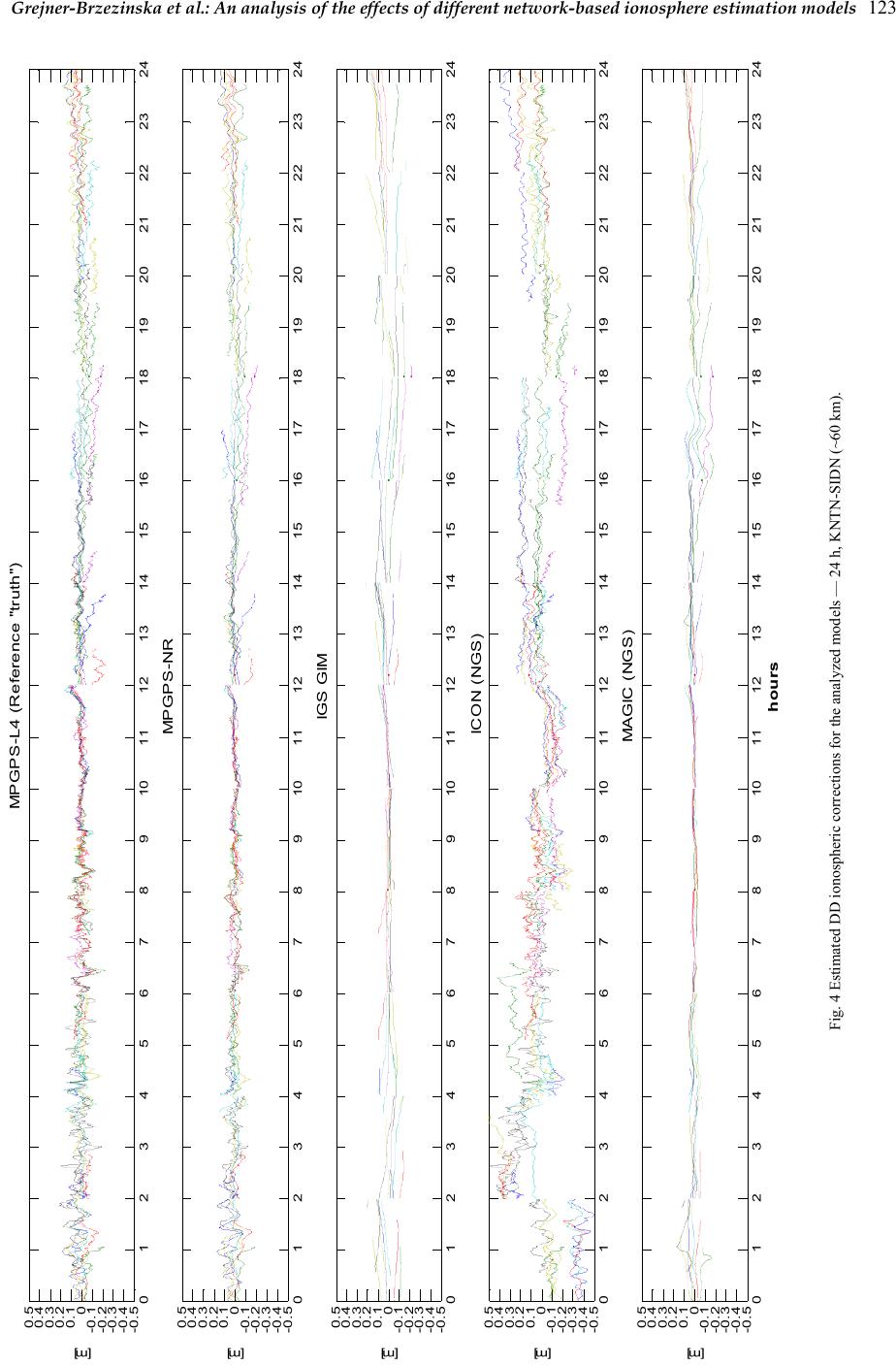

Grejner-Brzezinska et al.: An analysis of the effects of different network-based ionosphere estimation models 123
Fig. 4 Estimated DD ionospheric corrections for the analyzed models — 24 h, KNTN-SIDN (~60 km).
012345678910 11 12 13 14 15 16 17 18 19 20 21 22 2324
-0.5 -0.4 -0.3 -0.2 -0.1
0
0.1 0.2 0.3 0.4 0.5
MPGPS-L4 (Reference "truth")
[m]
012345678910 11 12 13 14 15 16 17 18 19 20 21 22 2324
-0.5 -0.4 -0.3 -0.2 -0.1
0
0.1 0.2 0.3 0.4 0.5
MPGPS-N R
[m]
012345678910 11 12 13 14 15 16 17 18 19 20 21 22 2324
-0.5 -0.4 -0.3 -0.2 -0.1
0
0.1 0.2 0.3 0.4 0.5
IGS GIM
[m]
012345678910 11 12 13 14 15 16 17 18 19 20 21 22 2324
-0.5 -0.4 -0.3 -0.2 -0.1
0
0.1 0.2 0.3 0.4 0.5
ICON (NGS)
[m]
012345678910 11 12 13 14 15 16 17 18 19 20 21 22 2324
-0.5 -0.4 -0.3 -0.2 -0.1
0
0.1 0.2 0.3 0.4 0.5
MAGIC (NGS)
[m]
hours

124 Journal of Global Positioning Systems
Fig. 5 DD ionospheric residuals with respect to the reference “truth” — 24 h, KNTN-SIDN (~60 km).
0 1 23 4 5 67 8 910 11 12 13 14 15 1617 18 1920 21 2223 24
-0.5 -0.4 -0.3 -0.2 -0.1
0
0.1 0.2 0.3 0.4 0.5
MPGPS-P4
[m]
0 1 23 4 5 67 8 910 11 12 13 14 15 1617 18 1920 21 2223 24
-0.5 -0.4 -0.3 -0.2 -0.1
0
0.1 0.2 0.3 0.4 0.5
MPGPS-NR
[m]
0 1 23 4 5 67 8 910 11 12 13 14 15 1617 18 1920 21 2223 24
-0.5 -0.4 -0.3 -0.2 -0.1
0
0.1 0.2 0.3 0.4 0.5
IGS GIM
[m]
0 1 23 4 5 67 8 910 11 12 13 14 15 1617 18 1920 21 2223 24
-0.5 -0.4 -0.3 -0.2 -0.1
0
0.1 0.2 0.3 0.4 0.5
ICON (NGS)
[m]
0 1 23 4 5 67 8 910 11 12 13 14 15 1617 18 1920 21 2223 24
-0.5 -0.4 -0.3 -0.2 -0.1
0
0.1 0.2 0.3 0.4 0.5
MAGIC (NGS)
[m]
hours

Grejner-Brzezinska et al.: An analysis of the effects of different network-based ionosphere estimation models 125
Fig. 6 Estimated DD ionospheric corrections for the analyzed models — 24 h, KNTN-DEFI (~100 km).
0 1 2 3 4 5 6 7 8 910 1112 13 14 15 16 17 18 19 20 21 22 2324
-0.5 -0.4 -0.3 -0.2 -0.1
0
0.1 0.2 0.3 0.4 0.5
MPGPS-L4 (Reference "truth")
[m]
0 1 2 3 4 5 6 7 8 910 1112 13 14 15 16 17 18 19 20 21 22 2324
-0.5 -0.4 -0.3 -0.2 -0.1
0
0.1 0.2 0.3 0.4 0.5
MPGPS-NR
[m]
0 1 2 3 4 5 6 7 8 910 1112 13 14 15 16 17 18 19 20 21 22 2324
-0.5 -0.4 -0.3 -0.2 -0.1
0
0.1 0.2 0.3 0.4 0.5
IGS GIM
[m]
0 1 2 3 4 5 6 7 8 910 1112 13 14 15 16 17 18 19 20 21 22 2324
-0.5 -0.4 -0.3 -0.2 -0.1
0
0.1 0.2 0.3 0.4 0.5
ICON (NGS)
[m]
0 1 2 3 4 5 6 7 8 910 1112 13 14 15 16 17 18 19 20 21 22 2324
-0.5 -0.4 -0.3 -0.2 -0.1
0
0.1 0.2 0.3 0.4 0.5
MAGIC (NGS)
[m]
hours

126 Journal of Global Positioning Systems
Fig. 7 DD ionospheric residuals with respect to the reference “truth” — 24 h, KNTN-DEFI (~100 km)
0 1 2 3 4 5 6 7 8 910 1112 13 14 15 16 17 18 19 20 21 22 2324
-0.5 -0.4 -0.3 -0.2 -0.1
0
0.1 0.2 0.3 0.4 0.5
MPGPS-P4
[m]
0 1 2 3 4 5 6 7 8 910 1112 13 14 15 16 17 18 19 20 21 22 2324
-0.5 -0.4 -0.3 -0.2 -0.1
0
0.1 0.2 0.3 0.4 0.5
MPGPS-NR
[m]
0 1 2 3 4 5 6 7 8 910 1112 13 14 15 16 17 18 19 20 21 22 2324
-0.5 -0.4 -0.3 -0.2 -0.1
0
0.1 0.2 0.3 0.4 0.5
IGS GIM
[m]
0 1 2 3 4 5 6 7 8 910 1112 13 14 15 16 17 18 19 20 21 22 2324
-0.5 -0.4 -0.3 -0.2 -0.1
0
0.1 0.2 0.3 0.4 0.5
ICON (NGS)
[m]
0 1 2 3 4 5 6 7 8 910 1112 13 14 15 16 17 18 19 20 21 22 2324
-0.5 -0.4 -0.3 -0.2 -0.1
0
0.1 0.2 0.3 0.4 0.5
MAGIC (NGS)
[m]
hours

Grejner-Brzezinska et al.: An analysis of the effects of different network-based ionosphere estimation models 127
44.25 4.5 4.7555.25 5.55.75 6
-0.2
-0.1
0
0.1
0.2
04:00 - 06:00 UTC
[m ]
1818.25 18.5 18.751919.25 19.519.7520
-0.2
-0.1
0
0.1
0.2
18:00 - 20:00 UTC
[m ]
hours
n
e
u
n
e
u
Fig. 8 Instantaneous RTK position residuals with respect to the known coordinates;
2-hour windows, KNTN-SIDN (~60 km); 0 cm constraint (1 sigma) was applied
to the ionospheric corrections.
44.25 4.54.7555.255.55.756
-0.2
-0.1
0
0.1
0.2
04:00 - 06:00 UTC
[m ]
1818.25 18.5 18.75 19 19.2519.5 19.7520
-0.2
-0.1
0
0.1
0.2
18:00 - 20:00 UTC
[m ]
hours
n
e
u
n
e
u
Fig. 9 Instantaneous RTK position residuals with respect to the known coordinates;
2-hour windows, KNTN-SIDN (~60 km); 5 cm constraint (1 sigma) was applied
to the ionospheric corrections.

128 Journal of Global Positioning Systems
44.25 4.54.7555.255.55.756
-0.2
-0.1
0
0.1
0.2
04:00 - 06:00 UTC
[m ]
1818.25 18.5 18.75 19 19.2519.5 19.7520
-0.2
-0.1
0
0.1
0.2
18:00 - 20:00 UTC
[m ]
hours
n
e
u
n
e
u
Fig. 10 Instantaneous RTK position residuals with respect to the known coordinates;
2-hour windows, KNTN-DEFI (~100 km); 0 cm constraint (1 sigma) was applied
to the ionospheric corrections.
44.25 4.54.7555.25 5.55.756
-0.2
-0.1
0
0.1
0.2
04:00 - 06:00 UTC
[m ]
n
e
u
1818.25 18.518.751919.25 19.519.7520
-0.2
-0.1
0
0.1
0.2
18:00 - 20:00 UTC
[m ]
hours
n
e
u
Fig. 11 Instantaneous RTK position residuals with respect to the known coordinates;
2-hour windows, KNTN-DEFI (~100 km); 1 cm constraint (1 sigma) for the ionospheric correction
was applied to the “best” window (bottom) and 5 cm for the “worst” window (top).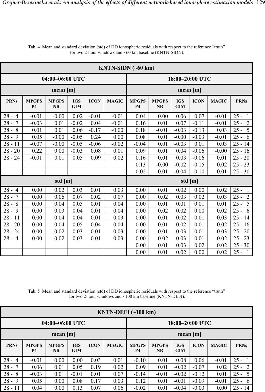

Grejner-Brzezinska et al.: An analysis of the effects of different network-based ionosphere estimation models 129
Tab. 4 Mean and standard deviation (std) of DD ionospheric residuals with respect to the reference “truth”
for two 2-hour windows and ~60 km baseline (KNTN-SIDN).
KNTN-SIDN (~60 km)
04:00–06:00 UTC 18:00–20:00 UTC
mean [m] mean [m]
PRNs MPGPS
P4
MPGPS
NR
IGS
GIM
ICON MAGIC MPGPS
P4
MPGPS
NR
IGS
GIM
ICON MAGIC PRNs
28 - 4 -0.01 -0.00 0.02 -0.01 -0.01 0.04 0.00 0.06 0.07 -0.01 25 - 1
28 - 7 -0.03 0.01 -0.02 0.04 -0.01 0.16 0.01 0.07 -0.11 -0.01 25 - 2
28 - 8 0.01 0.01 0.06 -0.17 -0.00 0.18 -0.01 -0.03 -0.13 0.03 25 - 5
28 - 9 0.05 -0.00 -0.05 0.24 0.00 0.08 0.01 -0.00 -0.03 -0.01 25 - 6
28 - 11 -0.07 -0.00 -0.05 -0.06 -0.02-0.04 0.01 -0.03 0.01 0.03 25 - 14
28 - 20 0.22 0.00 -0.03 0.08 0.01 0.09 0.01 0.04 -0.06 -0.00 25 - 16
28 - 24 -0.01 0.01 0.05 0.09 0.02 0.16 0.01 0.03 -0.06 0.01 25 - 20
0.13 -0.00 -0.02 -0.15 0.02 25 - 23
0.02 0.01 -0.04 -0.10 0.01 25 - 30
std [m] std [m]
28 - 4 0.00 0.02 0.03 0.01 0.030.00 0.01 0.02 0.00 0.02 25 - 1
28 - 7 0.00 0.06 0.07 0.02 0.070.00 0.02 0.03 0.02 0.03 25 - 2
28 - 8 0.00 0.04 0.05 0.01 0.040.00 0.01 0.01 0.01 0.01 25 - 5
28 - 9 0.00 0.03 0.04 0.01 0.040.00 0.02 0.02 0.00 0.02 25 - 6
28 - 11 0.00 0.04 0.04 0.01 0.030.00 0.01 0.02 0.01 0.03 25 - 14
28 - 20 0.00 0.04 0.05 0.04 0.040.00 0.01 0.02 0.01 0.02 25 - 16
28 - 24 0.00 0.02 0.03 0.01 0.030.00 0.01 0.03 0.01 0.03 25 - 20
28 - 4 0.00 0.02 0.03 0.01 0.030.00 0.02 0.03 0.01 0.02 25 - 23
0.00 0.01 0.03 0.02 0.02 25 - 30
0.00 0.01 0.02 0.00 0.02 25 - 1
Tab. 5 Mean and standard deviation (std) of DD ionospheric residuals with respect to the reference “truth”
for two 2-hour windows and ~100 km baseline (KNTN-DEFI).
KNTN-DEFI (~100 km)
04:00–06:00 UTC 18:00–20:00 UTC
mean [m] mean [m]
PRNs MPGPS
P4
MPGPS
NR
IGS
GIM
ICON MAGIC MPGPS
P4
MPGPS
NR
IGS
GIM
ICON MAGIC PRNs
28 - 4 -0.01 0.00 0.00 0.03 0.01-0.10 0.01 0.08 0.06 -0.01 25 - 1
28 - 7 0.06 0.01 0.05 0.19 0.02 0.09 0.01 -0.02 -0.07 0.02 25 - 2
28 - 8 -0.03 0.01 -0.01 0.01 0.07-0.14 -0.01 -0.02 -0.12 0.01 25 - 5
28 - 9 0.05 0.00 0.08 0.17 0.03 0.12 0.01 -0.01 -0.09 -0.01 25 - 6
28 - 11 0.04 0.00 0.13 0.07 0.06-0.02 0.01 -0.04 -0.03 0.00 25 - 14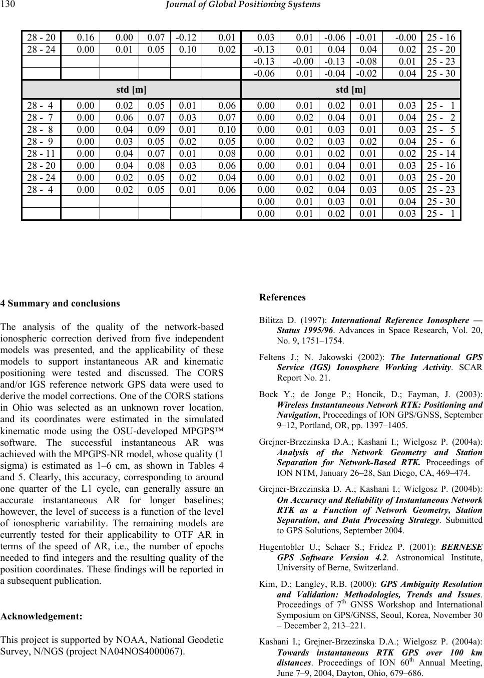

130 Journal of Global Positioning Systems
28 - 20 0.16 0.00 0.07 -0.12 0.01 0.03 0.01 -0.06 -0.01 -0.00 25 - 16
28 - 24 0.00 0.01 0.05 0.10 0.02-0.13 0.01 0.04 0.04 0.02 25 - 20
-0.13 -0.00 -0.13 -0.08 0.01 25 - 23
-0.06 0.01 -0.04 -0.02 0.04 25 - 30
std [m] std [m]
28 - 4 0.00 0.02 0.05 0.01 0.060.00 0.01 0.02 0.01 0.03 25 - 1
28 - 7 0.00 0.06 0.07 0.03 0.070.00 0.02 0.04 0.01 0.04 25 - 2
28 - 8 0.00 0.04 0.09 0.01 0.100.00 0.01 0.03 0.01 0.03 25 - 5
28 - 9 0.00 0.03 0.05 0.02 0.050.00 0.02 0.03 0.02 0.04 25 - 6
28 - 11 0.00 0.04 0.07 0.01 0.080.00 0.01 0.02 0.01 0.02 25 - 14
28 - 20 0.00 0.04 0.08 0.03 0.060.00 0.01 0.04 0.01 0.03 25 - 16
28 - 24 0.00 0.02 0.05 0.02 0.040.00 0.01 0.02 0.01 0.03 25 - 20
28 - 4 0.00 0.02 0.05 0.01 0.060.00 0.02 0.04 0.03 0.05 25 - 23
0.00 0.01 0.03 0.01 0.04 25 - 30
0.00 0.01 0.02 0.01 0.03 25 - 1
4 Summary and conclusions
The analysis of the quality of the network-based
ionospheric correction derived from five independent
models was presented, and the applicability of these
models to support instantaneous AR and kinematic
positioning were tested and discussed. The CORS
and/or IGS reference network GPS data were used to
derive the model corrections. One of the CORS stations
in Ohio was selected as an unknown rover location,
and its coordinates were estimated in the simulated
kinematic mode using the OSU-developed MPGPS
software. The successful instantaneous AR was
achieved with the MPGPS-NR model, whose quality (1
sigma) is estimated as 1–6 cm, as shown in Tables 4
and 5. Clearly, this accuracy, corresponding to around
one quarter of the L1 cycle, can generally assure an
accurate instantaneous AR for longer baselines;
however, the level of success is a function of the level
of ionospheric variability. The remaining models are
currently tested for their applicability to OTF AR in
terms of the speed of AR, i.e., the number of epochs
needed to find integers and the resulting quality of the
position coordinates. These findings will be reported in
a subsequent publication.
Acknowledgement:
This project is supported by NOAA, National Geodetic
Survey, N/NGS (project NA04NOS4000067).
References
Bilitza D. (1997): International Reference Ionosphere —
Status 1995/96. Advances in Space Research, Vol. 20,
No. 9, 1751–1754.
Feltens J.; N. Jakowski (2002): The International GPS
Service (IGS) Ionosphere Working Activity. SCAR
Report No. 21.
Bock Y.; de Jonge P.; Honcik, D.; Fayman, J. (2003):
Wireless Instantaneous Network RTK: Positioning and
Navigation, Proceedings of ION GPS/GNSS, September
9–12, Portland, OR, pp. 1397–1405.
Grejner-Brzezinska D.A.; Kashani I.; Wielgosz P. (2004a):
Analysis of the Network Geometry and Station
Separation for Network-Based RTK. Proceedings of
ION NTM, January 26–28, San Diego, CA, 469–474.
Grejner-Brzezinska D. A.; Kashani I.; Wielgosz P. (2004b):
On Accuracy and Reliability of Instantaneous Network
RTK as a Function of Network Geometry, Station
Separation, and Data Processing Strategy. Submitted
to GPS Solutions, September 2004.
Hugentobler U.; Schaer S.; Fridez P. (2001): BERNESE
GPS Software Version 4.2. Astronomical Institute,
University of Berne, Switzerland.
Kim, D.; Langley, R.B. (2000): GPS Ambiguity Resolution
and Validation: Methodologies, Trends and Issues.
Proceedings of 7th GNSS Workshop and International
Symposium on GPS/GNSS, Seoul, Korea, November 30
– December 2, 213–221.
Kashani I.; Grejner-Brzezinska D.A.; Wielgosz P. (2004a):
Towards instantaneous RTK GPS over 100 km
distances. Proceedings of ION 60th Annual Meeting,
June 7–9, 2004, Dayton, Ohio, 679–686.

Grejner-Brzezinska et al.: An analysis of the effects of different network-based ionosphere estimation models 131
Kashani I.; Wielgosz P.; Grejner-Brzezinska D.A. (2004b):
The Effect of Double-Difference Ionospheric
Corrections Latency on Instantaneous Ambiguity
Resolution in Long-Range RTK. ION GNSS 2004,
September 21–24, Long Beach, California, 2881–2890.
Odijk D. (2000): Weighting Ionospheric Corrections to
Improve Fast GPS Positioning Over Medium
Distances. Proceedings of ION GPS, September 19–22,
Salt Lake City, UT, 1113–1123.
Odijk D. (2001): Instantaneous GPS Positioning Under
Geomagnetic Storm Conditions. GPS Solutions, Vol. 5,
No. 2, 29–42.
Rizos C. (2002): Network RTK research and
implementation: A geodetic perspective. Journal of
Global Positioning Systems, Vol. 1, No. 2, 144–150.
Schaer S. (1999): Mapping and Predicting the Earth’s
Ionosphere Using the Global Positioning System. Ph.D.
Thesis, Astronomical Institute, University of Berne.
Schaer S.; Gurtner W.; Feltens J. (1998): IONEX The
IONosphere Map EXchange Format Version 1.
Proceedings of the IGS Analysis Center Workshop,
ESA/ESOC, February 9–11, Darmstadt, Germany, 233–
247.
Smith D.A. (2004): Computing unambiguous TEC and
ionospheric delays using only carrier phase data from
NOAA´s CORS network. Proceedings of IEEE PLANS
2004, April 26-29, Monterey, California, 527-537.
Spencer P.S.J.; Robertson D.S.; Mader, G.L. (2004):
Ionospheric data assimilation methods for geodetic
applications. Proceedings of IEEE PLANS 2004,
Monterey, California, April 26-29, 2004, 510-517.
Springer T.A. (1999): Modeling and Validating Orbits and
Clocks Using the Global Positioning System. Ph.D.
dissertation, Astronomical Institute, University of Berne,
Switzerland.
Teunissen P.J.G. (1994): A new method for fast carrier
phase ambiguity estimation. Proceedings of IEEE
PLANS’94, Las Vegas, NV, April 11–15, 562–573.
Teunissen P.J.G.; Joosten P.; Tiberius C. (2002): A
Comparison of TCAR, CIR and LAMBDA GNSS
Ambiguity Resolution. Proceedings of the ION GPS
2002, 24–27 September 2002, Portland, OR, 2799–2808.
Vollath U.; Buecherl A.; Landau H.; Pagels C.; Wagner B.
(2000): Multi-Base RTK Positioning Using Virtual
Reference Stations. Proceedings of ION GPS, 19–22
September 2000, Salt Lake City, UT, 123–131.
Wanninger L. (2002): Virtual Reference Stations for
Centimeter-Level Kinematic Positioning. Proceedings
of ION GPS 2002, September 24–27, Portland, Oregon,
1400–1407.
Wielgosz P.; Grejner-Brzezinska D.A.; Kashani I.; (2003):
Regional Ionosphere Mapping with Kriging and
Multiquadric Methods. Journal of Global Positioning
Systems, Vol. 2, Issue 1, 48–55.
Wielgosz P.; Grejner-Brzezinska D.; Kashani I. (2004):
Network Approach to Precise GPS Navigation.
Navigation, Vol. 51, No. 3, 213–220.