Journal of Modern Physics, 2012, 3, 1849-1855
http://dx.doi.org/10.4236/jmp.2012.312232 Published Online December 2012 (http://www.SciRP.org/journal/jmp)
Solutions of Schrödinger Equation with Generalized
Inverted Hyperbolic Potential
Akpan N. Ikot*, Eno J. Ibanga, Oladunjoye A. Awoga, Louis E. Akpabio, Akaninyene D. Antia
Theoretical Physics Group, Department of Physics, University of Uyo, Uyo, Nigeria
Received May 10, 2012; revised October 3, 2012; accepted October 18, 2012
ABSTRACT
The bound state solutions of the Schrödinger equation with generalized inverted hyperbolic potential using the Niki-
forov-Uvarov method are reported. We obtain the energy spectrum and the wave functions with this potential for arbi-
trary -state. It is shown that the results of this potential reduced to the standard potentials—Rosen-Morse, Poschl-
Teller and Scarf potential as special cases. We also discussed the energy equation and the wave function for these spe-
cial cases.
l

Keywords: Schrodinger Equation; Inverted Hyperbolic Potential; Nikiforov-Uvarov Method
1. Introduction
The analytical and numerical solutions of the wave equa-
tions for both relativistic and non-relativistic cases have
taken a great deal of interest recently. In many cases dif-
ferent attempts have been developed to solve the energy
eigenvalues from the wave equations exactly or numeri-
cally for non-zero angular momentum quantum number

0l

for a given potential [1-16]. It is well known that
these solutions play an essential role in the relativistic
and non-relativistic quantum mechanics for some physi-
cal potentials of interest, [1,2,12,17-19].
In this paper, we aim to solve the radial Schrödinger
equation for quantum mechanical system with inverted
generalized hyperbolic potential and show the results for
this potential using Nikiforov-Uvarov method (NU), [20].
The present paper is an attempt to carry out the ana-
lytical solutions of the Schrodinger equation with the
generalized inverted hyperbolic potential using the NU
method.
The hyperbolic potentials under investigations are
commonly used to model inter-atomic and intermolecular
forces [10,21]. Among such potentials are Poschl-Teller,
Rosen-Morse and Scarf potential, which have been stud-
ied extensively in the literatures, [5-8,22-25]. However,
some of these hyperbolic potentials are exactly solvable
or quasi-exactly solvable and their bound state solutions
have been reported, [3,4,11,13,26-28]. We seek to pre-
sent and study a generalized hyperbolic potential which
other potentials can be deduced as special cases within
the framework of Schrödinger equation with mass m and
potential V.
The paper is organized as follows: Section 2 is devoted
to the review of the Nikiforov-Uvarov method. In Sec-
tion 3 we present the exact solution of the Schrodinger
equation. Discussion and results are presented in Section
4. Finally we give a brief conclusion in Section 5.
2. Review of Nikiforov-Uvarov Method
The Nikiforov-Uvarov (NU) method, [20] was proposed
and applied to reduce the second order differential equa-
tion to the hypergeometric—type equation by an appro-
priate co-ordinate transformation S = S(r) as, [15,20].





 
20
ss
ss s
ss

 

 


(1)




where
s

and
s

are polynomials at most in the
second order, and

is a first order polynomial. In or-
der to find a particular solution of Equation (1) we use
the separation of variables with the transformation






s
ss   (2)
It reduces Equation (1) to an equation as hyper-
geometric type





 
0ss sss  
 


(3)


s
and 
is defined as a logarithmic derivative in the
following form and its solution can be obtained from





s

sπ
s
s


 (4)
*Corresponding author.
C
opyright © 2012 SciRes. JMP

A. N. IKOT ET AL. 1850
The other part of the wave formation


s

is the
function whose polynomial solu-hypergeometric type
tions are given by Rodriques relations.
   
d
d
nn
n
nn
B
s
ss
ss




(5)
where Bn is a normalization constant
nction

, and the weight
fu

s

must satisfy the condition.
 
d
d
s
s
s
   (6)
with
 
2π
s
ss  
nction

(7)
The fu

π
s
and trameter he pa

requires
ethod are definfor the NU med as follows:

2
π
22
s
k
 





 

 (8)

πks 
 
On the other hand in order to find the value of k, the
expression under the
square of polynomia
se
(9)
square root of Equation (8) must be
l. Thus, a new eigenvalue for the
cond order equation becomes


1
d
d2
n
nn
ns



 
  (10)
where tvative

he derid
d
s
s

is neg
Equati (10), we obtained the energy eigen-

ative. By comparing
ons (9) and
values.
3. Bound State Solutions of the Schrödinger
Equation
The Schrödinger equation with mass m and potential V(r)
takes the following form, [15]
 
2
20 m
rEVrr





 (11)
where the generalized hyperbolic potential V(r) under
investigation is defined as



2
,,, 01
2
2
coth coth
cosech
abcd
VraV rbVr
cVr d



 

(12)
Here V0, V1 and V2 are the depth of the potential and a,
b, c and d are real numbers. The generalized hyperbolic
potential V(r) of Equation (12) has the following special
cases:




2
,0, ,002
coth cosech
ac
VraV rcVr


 (13) (i)


2
0,0, ,02cosech c
VrcV r

 (14) (ii)




2
0, ,0,0coth b
Vrb r


 
(15) (iii)
The potentials (13)-(15) are the Rosen-Morse poten-
tial, Poschl-Teller potential and Scarf potential respec-
tively.
We now perform the transformation [6,7,15]

Rr
rr 

(16)
on Equation (1) and obtain
 
22
2
coth cothcosech0RrEaVrbVr cVr dRr  
    (17)
where the prime indicates differentiation both respect to
r.
Now using a new ansaltz for the wave function in the

01
2
h
2m
form [3,4,11]

2
e
r
Rr Fr



and including the centrifugal term, reduces Equation (17)
into the following differential equat
(18)
ion,
  
2
2
22
1
cosech 0
l
cVr dFr
r




 


 (19)
2
2
2
dd2 coth coth
d
Rr Fm
EaVr bV
r


 

01
2
d2
r
rh



Because of the centrifugal term in Equation (19), this
ytically when the angular
. Therefore, in order
centrifugal term. Thus, when 1r

 we us
proximation scheme [9,29] for the centrifugal te
equation cannot be solved anal
omentum quantum number 0
to
m
find the approximate analytical solution of Equation
(19) with 0, we must make an approximation for the
e the ap-
rm,

22
2cosech
r

1r


get
 (20)
Substituting Equation (20) into Equation (19), we
 
 
2
2
22 22
01 2
2
2cothcothcosech1 cosech0 mEaVrbVrcVrllrdFr   
 

  
 
 

)
2
dd
dd
Fr Fr
rr


h




(21

A. N. IKOT ET AL. 1851
Now making the change of variable


coth
s
r


we obtain
(22)
 





22
2 2
01 2
11
1 0
a
VsbVscVsllsdFs




2
2
22
2
22
dd
2
d
2
2
FF
ss
s
mE












(23)
Simplifying Equation (23), we have
2
11
d
s
s

 

220ss
Fs 



wmeters have been
employed:
2
22
22
22
d2d1
dd 11
FsF
ss ss
 

 (24)


here the following dimensionless para




1d

 


 ,
22
2
22
2
2
mEcV 




 




2
2,1 ,
s
20
2maV

22




22
21 m
  25)
Comparing Equations (1) and (24), we obtain the fol-
lowing polynomials,
21
22cV bV



 (
22 22
.
ss s
s


 (26)
Substituting these polynomials into Equation (8), we
obtain the π()
s s     
s
function as


2222 2
44 44 4
2kss k
π
2
1
s

 

The expon in the square r

(27)
ressioot of Equation (27)
must be square of polynomial in respect of the NU
method. Therefore, we determine the


π
s
-valu

es as

uvs u

v


2
22 22
2
2
rku
v



22 22
,fo
π
2o2
,f r
2uvs uv
s
kuv



1uv
s uv




 







 




) (28
where
2
22
2
1a
2
uV

22
5
nd 2 i

   .
For the polynomial of






2π

  which has a nega-
get tive derivative, we
2


22 22
2
kuv
  
 9)
 (2
 
1
π
22
s
uvs uv


 

(30)  
Now using


πks 

 , we obtain


s

and

valued as
 
2
s
suvsuv    (31)

2
22 22
1
22
s
uv    (3) uv



 

 2
Another definition of n

is as given in Equation (10),
thus using values of


d


s
 , we get,
s
 an

1
nuuv uu


 (33)
Comparing Equations (32) and (33), we obtain the en-
value equation as ergy eigen




21
1
i 
 

42
4
2
111
24
82 82
110
2
niv
v
ni
vivn i


22
2
 
 
 

 


  
  


  

where

(34)


21
2nn

2





 .
ob
Solving the energy eiginvalue equation explicitly, we
tain the energy eiginvalues as

A. N. IKOT ET AL. 1852
 

 

21i



2
2
2
4
2
11
41
11 1
11
11
22
22
82 8282 8
11
22
22
vn
i
nn
ii
vv
r
nv i
iVn i


 
 


 
11 4
42
82 82
i
vv
 

2





 

  


 


 





 


 

 

 

 



 



(35)
Now using these quantities of Equation (20) and the definition for


and V given as
 
22 1
22
nn
m






(36)
2
0
21
22
21 av mcV bV l


  


2
021
22
21 m
Vi aVcVbV





 
 (37) for the Schrödinger equa
We obtain the energy spectrum of the Equation (35)
tion with the generalized in-
verted hyperbolic potential as

 



21
11
n
2
22 222
2
2
11 4
11 4
24 82 82
2
11
11
22
22
82 8282
2
nl
ir
ii
vvv
mr
m
Enn
r
i
v
rr
cV

 
 

4
2
11
22
22
nri
r
xvivnir
v

82
r
i




 
 
 


 


 

  





  






  
 

  






 









21d
 
We now find the corresponding eigenfunctions. The
polynomial solutions of the hyperbolic function
(38)


n
s

depend on the determination of weight function


s
 .
Thus we determine the


s
 function in Equation (6)
as


2
21
1
iv
is
ss





 
(39)
1is

where 2uv   , uv
 
and subst
Equation (39) in to the Rodriques relation of Equati),
we have
ituting
on (5
 

1
d
nn
n
sB

22 2i
2
1
d
Ni n
is lis
is
s
i 2 v
1
nis



 
 




  (40)




The polynomial solution of

n
s

can be expressed
in terms of Jacobi polynomials which is one of the or-
thogonal polynomials, which is


2,2AA
n
x

 , where
A
i

  , and
x
is.
The other part of the wave
Equation (4) as,
function is obtain from
 
22
11
B
B
is
 

where
sis   (41)
.
2
Bi



Combining the Jacobi polynomials of Equations (40)
and (41), we obtain the redial wave function of the
Schrödinger equation with inverted generalized hyper-
bolic potential as
  
2,2
22
11
BB
AA
nl nn
F
SNxx Px
 

Nn i
co
2()d 1
n
Rss

 
.
The total radial wave function is obta
tions (18) and (22) as
 
  (43)
where s a new normalization constant and obeys the
ndition
in using Equa-
   
2,
2
2
1icothicoth
nl n
BAA
n
rr
P





(43)
4. Results and D
2
1icoth
B
N r




iscussion
The well-known potentials are obtained from th
Rr
e gener-
alized inverted hyperbolic potential if we make appropri-

A. N. IKOT ET AL. 1853
ate choose for the values of the parameters in the gener-
alized inverted potentials as stated in Section 3. We plot-
ted the variation of the generalized inverted hyperbolic
po
2
1,2,3and4 as display in
Figure 1.
Rosen-Morse Potential: For b = d = 0, the
Morse Potential is obtain as given in Equation (13). We
plotted the variation of Rosen-Morse V(r) with r for a =
.02 MeV with different
tential as a function of r for a = 1, b = 0.01, V0 = 1
MeV, V1 = 0.5 MeV, C = 2, V = 0.02 MeV, d = 2 MeV
at different parameters of
2

Rosen-
–1, V0 = 1 MeV, c = 2 and V2 = 0

parameters of 1,2, 3and
 4 in Figure 2. Substi-
02 MeV in Fig
e parameters in the energy equation of Equa-
tio
tuting b = d = 0 in Equations (38) and (43), we obtain the
energy spectrum and the wave function of the Rosen-
Morse potential respectively.
Poschl-Teller Potential: Poschl-Teller Potential is
obtain from the generalized inverted hyperbolic potential
by setting a = b = d = 0 and c = –c as given in Equation
(14). The Poschl-Teller potential is plotted as a function
of r for c = –2 and V2 = 0.ure 3. Substi-
tuting thes
n (38) and wave function (43), we obtain the desired
Figure 1. A plot of inverted generalized hyperbolic poten-
rial with r for a = 1, b = 0.01, c = 2, d = 2 MeV, V0 = 1 MeV,
V1 = 0.5 MeV, V2 = 0.02 MeV and α = 1, 2, 3, and 4.
Figure 2. Variation of Rosen-Morse potential with r for a =
1, b = 0, c = 2, d = 0, V0 = 1 MeV, V2 = 0.02 MeV with
various parameter of α = 1, 2, 3, and 4.
energy spectrum and the wave function of the Poschl-
Teller potential.
Scarf Potential: We can deduce the Scarf potential
from the generalized inverted hyperbolic potential by
setting a = c = d = 0. We display in Figure 4 the plot of
Scarf potential as a function of r for b = 0.05, V1 = 0.5
MeV with various parameter of 1,2, 3and4
 . Setting
the above limiting values in Equations (38) and (43) we
obtain the energy eigen-values and wave function for the
Scarf potential respectively.
5. Conclusion
–
The bound state solutions of the Schrödinger equation
with a generalized inverted hyperbolic potential have
been investigated within the framework of the NU me-
thod. Three well-known potential have been deduced
from this potential. We discussed the energy spectrum
and the wave function of the SE with this potential for an
arbitrary l-state. We also discussed the special cases of
the generalized inverted hyperbolic potential: Rosen
Morse, Poschl-Teller and Scarf potentials. Finally, we
plotted the effective potential as a function of r for dif-
ferent l = 1, 2, 3 and 4 as shown in Figure 5.
Figure 3. A plot of Poschl-Teller potenrial with r for 0.01, c
= −2, V2 = 0.02 MeV with various parameter of α = 1, 2, 3,
and 4.
Figure 4. A plot of Scarf potenrial with r for a = 0, b = 0.05,
c = 0, d = 0, V1 = 0.5 MeV with various parameter of α = 1, 2,
3, and 4.

A. N. IKOT ET AL. 1854
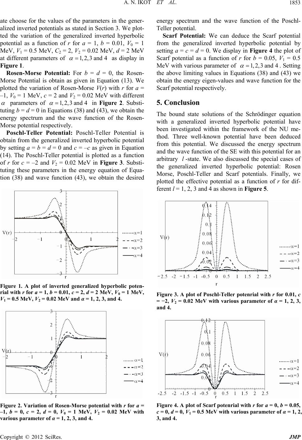
Figure 5. A variation of the effective potential as a function
of r for l = 1, 2, 3 and 4 with α = 1.
k is partially supported by the Nandy Resea
Grant No. 64-01-2271.
REFERENCES
[1] O. M. Al-Dossary, “Morse Potential Eigen-Energies
through the Asymptotic Iteration Method,” International
Journal of Quantum Chemistry, Vol. 107, No. 10, 2007
pp. 2040-2046. doi:10.1002/qua.21335
6. Acknowledgements
This worrch
,
[2] Y. F. Cheng and T. Q. Dai, “Exact Solutions of the Klein-
Gordon Equation with a Ring-Shaped Modified Kratze
Potential,” Chinese Journal of Physics, Vol. 45, No. 5,
ch, “Trigonometric Quark
QCD Traits,” The European
3, No. 1, 2007, pp. 1-4.
r
2007, p. 480.
[3] C. B. Compean and M. Kirchba
Confinement Potential of
Physical Journal A, Vol. 3
doi:10.1140/epja/i2007-10444-0
[4] C. B. Compean and M. Kirchbach, “The Trigonometric
Rosen-Morse Potential in the Supersymmetric Quantum
Mechanics and Its Exact Solutions,” Journal of Physics A
Vol. 39, No. 3
doi:10.1088/030
,
, 2006, p. 547.
5-4470/39/3/007
[5] A. Contreras-Astorga and D. J. Fernandez, “Supersym-
metric Partners of the Trigonometric Poschl-Teller Poten-
tials,” Journal of Physics A, Vol. 41, No. 47, 2008, Arti-
cle ID: 475303.
[6] F. Cooper, A. Khare and U. Sukhature, “Supersymmetry
and Quantum Mechanics,” Physics Reports, Vol. 251, No.
5-6, 1990, pp. 267-385.
doi:10.1016/0370-1573(94)00080-M
, 1999,
2/48/308
[7] J. J. Diaz, J. Negro, I. M. Nieto and O. Rosas, “The Su-
persymmetric Modified Poschl-Teller and Delta-Well
Potentials,” Journal of Physics A, Vol. 32, No. 48
p. 8447. doi:10.1088/0305-4470/3
” Journal of Physics A
, Article ID: 358198.
cal Physics, Vol. 50, 2011, pp.
[8] D. J. Fernandez, “Supersymmetric Quantum Mechanics,”
arxiv: 0910.0192v1, 2009.
[9] R. I. Greene and C. Aldrich, “Variational Wave Function
for a Screened Coulomb Potential,,
Vol. 14, No. 6, 1976, pp. 2363-2366.
[10] A. S. Halberg, “Quasi-Exact Solvability of a Hyperbolic
Intermolecular Potential Induced by an Effective Mass
Step,” International Journal Mathematics and Mathe-
matical Sciences, Vol. 2011
[11] S. D. Hernandez and D. J. Fernandez, “Rosen-Morse
Potentials and Its Supersymmetric Partners,” Interna-
tional Journal of Theoreti
1993-2001.
[12] S. Ikhdair and R. Sever, “Polynomial Solutions of Non-
Central Potentials,” International Journal of Theoretical
Physics, Vol. 46, No. 10, 2002, pp. 2384-2395.
doi:10.1007/s10773-007-9356-8
[13] A. N. Ikot and L. E. Akpabio, “Approximate Solution of
Schrodinger Equation with Rosen-Morse Potential In-
. D. Agboola, “Ex-
cluding a Centrifugal Term,” Applied Physics Research,
Vol. 2, No. 2, 2010, p. 202.
[14] K. J. Oyewumi, E. O. Akinpelu and A
actly Complete Solutions of the Pseudoharmonic Poten-
tial in N-Dimensions,” International Journal of Theo-
retical Physics, Vol. 47, No. 4, 2008, pp. 1039-1057.
doi:10.1007/s10773-007-9532-x
[15] R. Sever, C. Tezcan, O. Yesiltas and M. Bucurget, “Exact
Solution of Effective Mass Schrodinger Equation for the
Hulthen Potential,” International Journal of Theoretical
Physics, Vol. 47, No. 9, 2008, pp. 2243-2248.
doi:10.1007/s10773-008-9656-7
[16] G. F. Wei, X. Y. Liu and W. L. Chen, “The Relativistic
Scattering States of the Hulthen Potential with an Im-
proved New Approximation Scheme to the C
Term,” International Journal of Tentrifugal heoretical Physics, Vol.
48, No. 6, 2009, pp. 1649-1658.
doi:10.1007/s10773-009-9937-9
[17] H. X. Quan, L. Guang, W. Z. Min, N. L. Bin and M. Yan,
“Solving Dirac Equation with New Ring-Shaped Non-
Spherical Harmonic Oscillator,” Communications in The o-
retical Physics, Vol. 53, No. 2, 2010, p. 242.
doi:10.1088/0253-6102/53/2/07
[18] A. N. Ikot, A. D. Antia, L. E. Akpabio and J. A. O
“Analytic Solutions of Schroding
bu,
ound State
uation with Hulthen Po-
Solutions
of Physics,
o the
er Equation with Two-
Dimensional Harmonic Potential in Cartesian and Polar
Coordinates via Nikiforov-Uvarov Method,” Journal of
Vectorial Relativity, Vol. 6, No. 2, 2011, pp. 65-76.
[19] A. N. Ikot, L. E. Akpabio and E. J. Uwah, “B
Solution of the Klein-Gordon Eq
tential,” Electronic Journal of Theoretical Physics, Vol. 8,
No. 25, 2011, pp. 225-232.
[20] A. F. Nikiforov and U. B. Uvarov, “Special Functions of
Mathematical Physics,” Birkhausa, Basel, 1988.
[21] A. N. Ikot, L. E. Akpabio and J. A. Obu, “Exact
of Schrodinger Equation with Five-Parameter Potential,”
Journal of Vectorial Relativity, Vol. 6, No. 1, 2011, p. 1.
[22] S. Meyur and S. Debnath, “Lie Algebra Approach to Non-
Hermitian Hamiltonians,” Bulgarian Journal
Vol. 36, No. 2, 2009, pp. 77-87.
[23] S. Meyur, “Algebraic Aspect for Two Solvable Poten-
tials,” Electronic Journal of Theoretical Physics, Vol. 8,
No. 25, 2011, pp. 217-224.
[24] S. G. Roy, J. Choudhury, N. K. Sarkar, S. R. Karumuri
and R. Bhattacharjee, “A Lie Algebra Approach t
Schrodinger Equation for Bound States of Poschl-Teller

A. N. IKOT ET AL. 1855
. Cui, “Approximate Analytic
pin-Cen-
Potential,” Electronic Journal of Theoretical Physics, Vol.
7, No. 24, 2010, pp. 235-240.
[25] C. S. Jia, T. Chen and L. G
Solutions of the Dirac Equation with the Generalized
Poschl-Teller Potential Including the Pseudo-S
trifugal Term,” Physics Letters A, Vol. 373, 2009, pp.
1621-1626. doi:10.1016/j.physleta.2009.03.006
[26] K. J. Oyewumi and C. O. Akoshile, “Bound State Solu-
tions of the Dirac-Rosen-Morse Potential with Spin and
Pseudospin Symmetry,” The European Physical Journal
A, Vol. 45, 2010, pp. 311-318.
doi:10.1140/epja/i2010-11007-0
[27] K. J. Oyewumi, “Analytic Solution of the Kratzer-Feus
Potential in an Arbitrary Number of Dimensions,” Foun-
dations of Physics Letters, Vol. 18, No. 75, 2005.
[28] W. A. Yahya, K. J. Oyewumi, C. O. Akoshile and T. T.
0, pp. 1-8.
roximate Analytical So-
Ibrahim, “Bound State Solutions of Relativistic Dirac
Equation with Equal Scalar and Vector Eckart Potentials
Using the Nikivorov-Uvarov Method,” Journal of Vecto-
rial Relativity, Vol. 5, No. 3, 201
[29] Y. Xu, S. He and C. S. Jia, “App
lutions of the Klein-Gordon Equation with Poschl-Teller
Potential Including the Centrifugal Term,” Physica Scripta,
Vol. 81, No. 4, 2010, Article ID: 045001.
doi:10.1088/0031-8949/81/04/045001