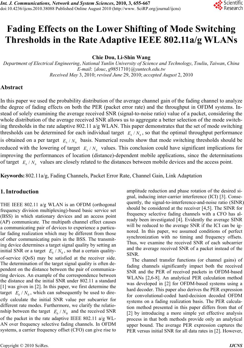Int. J. Communications, Network and System Sciences, 2010, 3, 655-667
doi:10.4236/ijcns.2010.38088 Published Online August 2010 (http://www. SciRP.org/journal/ijcns)
Fading Effects on the Lower Shifting of Mode Switching
Thresholds in the Rate Adaptive IEEE 802.11a/g WLANs
Chie Dou, Li-Shin Wang
Department of Electrical Engineering, National Yunlin University of Science and Technology, Touliu, Taiwan, China
Received May 3, 2010; revised June 29, 2010; accepted August 2, 2010
Abstract
In this paper we used the probability distribution of the average channel gain of the fading channel to analyze
the degree of fading effects on both the PER (packet error rate) and the throughput in OFDM systems. In-
stead of solely examining the average received SNR (signal-to-noise ratio) value of a packet, considering the
whole distribution of the average received SNR allows us to aggregate a better selection of the mode switch-
ing thresholds in the rate adaptive 802.11 a/g WLAN. This paper demonstrates that the set of mode switching
thresholds can be determined for each individual target , so that the optimal throughput performance
is obtained on a per target basis. Numerical results show that mode switching thresholds should be
reduced with the lowering of target values. This conclusion could have significant implications for
improving the performances of location (distance)-dependent mobile applications, since the determinations
of target values are closely related to the distances between mobile devices and the access point.
0
/NEb
0
/NEb
0
/NEb
0
/NEb
Keywords: 802.11a/g, Fading Channels, Packet Error Rate, Channel Gain, Link Adaptation
1. Introduction
THE IEEE 802.11 a/g WLAN is an OFDM (orthogonal
frequency division multiplexing)-based basic service set
(BSS) in which stationary devices and an access point
(AP) communicate. The multipath channel effect causes
a communicating pair of devices to experience a particu-
lar fading realization which may be different from those
of other communicating pairs in the BSS. The transmit-
ing device determines a target signal quality by setting an
initial SNR or a target , so that a certain quality-
of-service (QoS) may be satisfied at the receiver side.
The determination of the target signal quality is often de-
pendent on the distance between the pair of communica-
ting devices. An example of the correspondence between
the distance and the initial SNR under 802.11 a standard
[1] was given in [2]. In this paper, we first determine the
target , which can subsequently be used to dire-
ctly calculate the initial SNR value per subcarrier for
different rate modes. Furthermore, we clarify the relatio-
nship between the target and the received SNR
of the packet in the rate adaptive IEEE 802.11 a/g WL-
AN over frequency selective fading channels. In OFDM
systems, a carrier frequency offset (CFO) can give rise to
amplitude reduction and phase rotation of the desired si-
gnal, inducing inter-carrier interference (ICI) [3]. Conse-
quently, the signal-to-interference-and-noise ratio (SINR)
should be considered at the receiver [4,5]. The SINR for
frequency selective fading channels with a CFO has al-
ready been investigated [4]. Evidently the average SINR
will be reduced to the average SNR if the ICI can be ig-
nored. In this paper, we assumed conditions of perfect
synchronization with no timing and frequency offsets.
Thus, we examine the received SNR of each subcarrier
and the average received SNR of a packet instead of the
SINR.
0
/NEb
/NEb
0
/NEb
0
The channel transfer functions (or channel gains) of
fading channels significantly impact both the received
SNR and the PER of received packets in OFDM-based
WLANs [2,6-8]. An analytical PER calculation method
was developed in [2] for OFDM-based systems using a
hard decoder. This paper also derives the PER expression
for convolutional-coded hard-decision decoded OFDM
systems on a fading realization basis. The PER calcula-
tion method presented in this paper differs from that of
[2] by introducing a more simple yet effective analysis
process in that both methods provide only an analytical
upper bound. The average PER expression captures the
PER versus initial SNR for all data rates in [2]. However,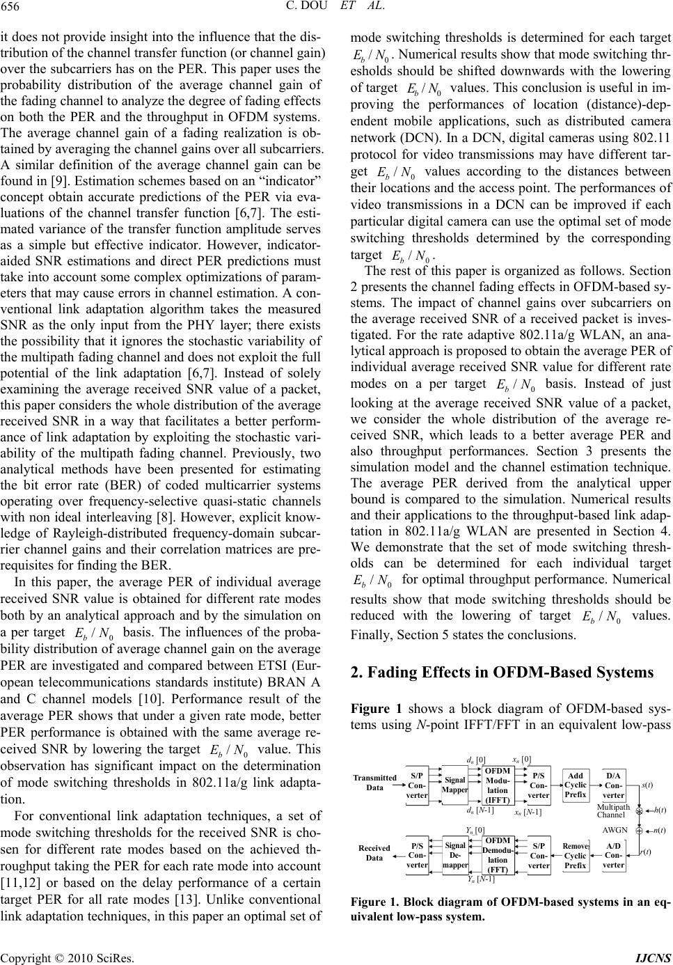

656 C. DOU ET AL.
it does not provide insight into the influence that the dis-
tribution of the channel transfer function (or channel gain)
over the subcarriers has on the PER. This paper uses the
probability distribution of the average channel gain of
the fading channel to analyze the degree of fading effects
on both the PER and the throughput in OFDM systems.
The average channel gain of a fading realization is ob-
tained by averaging the channel gains over all subcarriers.
A similar definition of the average channel gain can be
found in [9]. Estimation schemes based on an “indicator”
concept obtain accurate predictions of the PER via eva-
luations of the channel transfer function [6,7]. The esti-
mated variance of the transfer function amplitude serves
as a simple but effective indicator. However, indicator-
aided SNR estimations and direct PER predictions must
take into account some complex optimizations of param-
eters that may cause errors in channel estimation. A con-
ventional link adaptation algorithm takes the measured
SNR as the only input from the PHY layer; there exists
the possibility that it ignores the stochastic variability of
the multipath fading channel and does not exploit the full
potential of the link adaptation [6,7]. Instead of solely
examining the average received SNR value of a packet,
this paper considers the whole distribution of the average
received SNR in a way that facilitates a better perform-
ance of link adaptation by exploiting the stochastic vari-
ability of the multipath fading channel. Previously, two
analytical methods have been presented for estimating
the bit error rate (BER) of coded multicarrier systems
operating over frequency-selective quasi-static channels
with non ideal interleaving [8]. However, explicit know-
ledge of Rayleigh-distributed frequency-domain subcar-
rier channel gains and their correlation matrices are pre-
requisites for finding the BER.
In this paper, the average PER of individual average
received SNR value is obtained for different rate modes
both by an analytical approach and by the simulation on
a per target 0 basis. The influences of the proba-
bility distribution of average channel gain on the average
PER are investigated and compared between ETSI (Eur-
opean telecommunications standards institute) BRAN A
and C channel models [10]. Performance result of the
average PER shows that under a given rate mode, better
PER performance is obtained with the same average re-
ceived SNR by lowering the target 0 value. This
observation has significant impact on the determination
of mode switching thresholds in 802.11a/g link adapta-
tion.
/NEb
/NEb
For conventional link adaptation techniques, a set of
mode switching thresholds for the received SNR is cho-
sen for different rate modes based on the achieved th-
roughput taking the PER for each rate mode into account
[11,12] or based on the delay performance of a certain
target PER for all rate modes [13]. Unlike conventional
link adaptation techniques, in this paper an optimal set of
mode switching thresholds is determined for each target
0. Numerical results show that mode switching thr-
esholds should be shifted downwards with the lowering
of target 0 values. This conclusion is useful in im-
proving the performances of location (distance)-dep-
endent mobile applications, such as distributed camera
network (DCN). In a DCN, digital cameras using 802.11
protocol for video transmissions may have different tar-
get 0 values according to the distances between
their locations and the access point. The performances of
video transmissions in a DCN can be improved if each
particular digital camera can use the optimal set of mode
switching thresholds determined by the corresponding
target .
/NEb
/Eb
/NEb
N
/N0b
The rest of this paper is organized as follows. Section
2 presents the channel fading effects in OFDM-based sy-
stems. The impact of channel gains over subcarriers on
the average received SNR of a received packet is inves-
tigated. For the rate adaptive 802.11a/g WLAN, an ana-
lytical approach is proposed to obtain the average PER of
individual average received SNR value for different rate
modes on a per target basis. Instead of just
looking at the average received SNR value of a packet,
we consider the whole distribution of the average re-
ceived SNR, which leads to a better average PER and
also throughput performances. Section 3 presents the
simulation model and the channel estimation technique.
The average PER derived from the analytical upper
bound is compared to the simulation. Numerical results
and their applications to the throughput-based link adap-
tation in 802.11a/g WLAN are presented in Section 4.
We demonstrate that the set of mode switching thresh-
olds can be determined for each individual target
for optimal throughput performance. Numerical
results show that mode switching thresholds should be
reduced with the lowering of target values.
Finally, Section 5 states the conclusions.
E
0
/NEb
0
/NEb
0
/NEb
2. Fading Effects in OFDM-Based Systems
Figure 1 shows a block diagram of OFDM-based sys-
tems using N-point IFFT/FFT in an equivalent low-pass
Transmitted
Data
Received
Data
S/P
Con-
verter
P/S
Con-
verter
Signal
Mapper
Signal
De-
ma
pp
er
OFDM
Modu-
lation
(IFFT)
OFDM
Demodu-
lation
(FFT)
P/S
Con-
verter
S/P
Con-
verter
Add
Cyclic
Prefix
Remove
Cyclic
Prefix
D/A
Con-
verter
A/D
Con-
verter
dn [0]
x
n [0]
dn [N-1]
x
n [N-1]
Yn [N-1]
Yn [0]
Multip a t h
Channel
AWGN
s(t)
h(t)
n(t)
r(t)
Figure 1. Block diagram of OFDM-based systems in an eq-
uivalent low-pass system.

C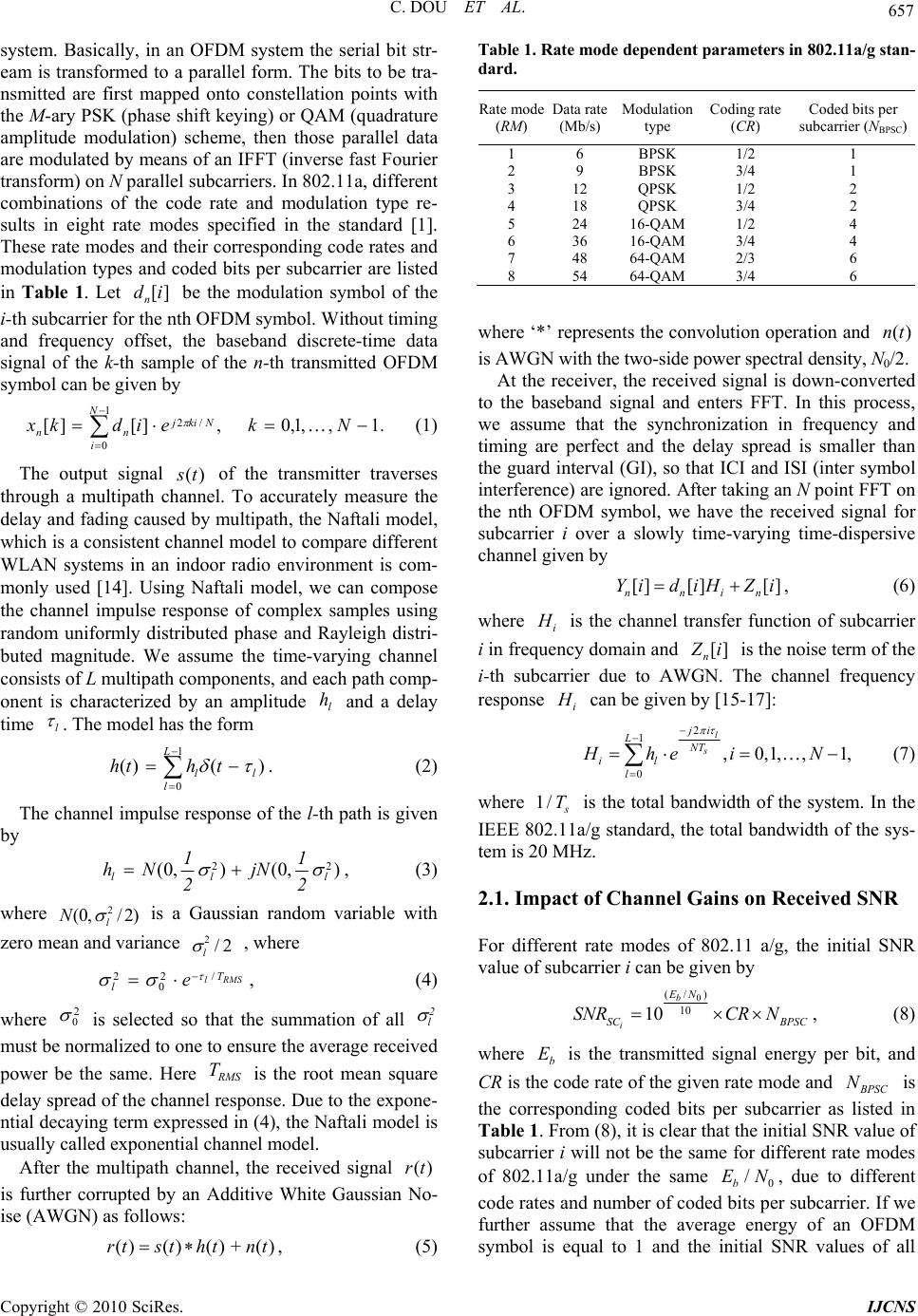. DOU ET AL.
657
system. Basically, in an OFDM system the serial bit str-
eam is transformed to a parallel form. The bits to be tra-
nsmitted are first mapped onto constellation points with
the M-ary PSK (phase shift keying) or QAM (quadrature
amplitude modulation) scheme, then those parallel data
are modulated by means of an IFFT (inverse fast Fourier
transform) on N parallel subcarriers. In 802.11a, different
combinations of the code rate and modulation type re-
sults in eight rate modes specified in the standard [1].
These rate modes and their corresponding code rates and
modulation types and coded bits per subcarrier are listed
in Table 1. Let be the modulation symbol of the
i-th subcarrier for the nth OFDM symbol. Without timing
and frequency offset, the baseband discrete-time data
signal of the k- th sample of the n-th transmitted OFDM
symbol can be given by
][idn
.1,,1,0,][][
1
0
/2  


Nk eidkx
N
i
Nkij
nn 

(1)
The output signal of the transmitter traverses
through a multipath channel. To accurately measure the
delay and fading caused by multipath, the Naftali model,
which is a consistent channel model to compare different
WLAN systems in an indoor radio environment is com-
monly used [14]. Using Naftali model, we can compose
the channel impulse response of complex samples using
random uniformly distributed phase and Rayleigh distri-
buted magnitude. We assume the time-varying channel
consists of L multipath components, and each path comp-
onent is characterized by an amplitude and a delay
time
)(ts
l
h
l

. The model has the form



0
)()(
l
ll thth

1L
. (2)
The channel impulse response of the l-th path is given
by
),0(),0( 22
lll 2
1
jN
2
1
Nh   , (3)
where )2/ ,0(2
l
N

is a Gaussian random variable with
zero mean and variance 2/2
l

, where
RMSl T
le/
2
0
2




 , (4)
where is selected so that the summation of all
2
0

2
l

must be normalized to one to ensure the average received
power be the same. Here is the root mean square
delay spread of the channel response. Due to the expone-
ntial decaying term expressed in (4), the Naftali model is
usually called exponential channel model.
RMS
T
After the multipath channel, the received signal
is further corrupted by an Additive White Gaussian No-
ise (AWGN) as follows:
()rt
()()() + ()rt st htnt , (5)
Table 1. Rate mode dependent parameters in 802.11a/g stan-
dard.
Rate mode
(RM)
Data rate
(Mb/s)
Modulation
type
Coding rate
(CR)
Coded bits per
subcarrier (NBPSC)
1 6 BPSK 1/2 1
2 9 BPSK 3/4 1
3 12 QPSK 1/2 2
4 18 QPSK 3/4 2
5 24 16-QAM1/2 4
6 36 16-QAM3/4 4
7 48 64-QAM2/3 6
8 54 64-QAM3/4 6
where ‘*’ represents the convolution operation and
is AWGN with the two-side power spectral density, N0/2.
()nt
At the receiver, the received signal is down-converted
to the baseband signal and enters FFT. In this process,
we assume that the synchronization in frequency and
timing are perfect and the delay spread is smaller than
the guard interval (GI), so that ICI and ISI (inter symbol
interference) are ignored. After taking an N point FFT on
the nth OFDM symbol, we have the received signal for
subcarrier i over a slowly time-varying time-dispersive
channel given by
[] [][]
nnin
YidiH Zi

, (6)
where i
H
is the channel transfer function of subcarrier
i in frequency domain and []
n
Z
i is the noise term of the
i-th subcarrier due to AWGN. The channel frequency
response i
H
can be given by [15-17]:
2
1
0
,0,1,, 1
l
s
ji
LNT
il
l
Hhe iN
 


,



(7)
where 1/
s
T is the total bandwidth of the system. In the
IEEE 802.11a/g standard, the total bandwidth of the sys-
tem is 20 MHz.
2.1. Impact of Channel Gains on Received SNR
For different rate modes of 802.11 a/g, the initial SNR
value of subcarrier i can be given by
0
(/ )
10
10
b
i
EN
SC BPSC
SNRCR N, (8)
where is the transmitted signal energy per bit, and
CR is the code rate of the given rate mode and
b
E
B
PSC
N is
the corresponding coded bits per subcarrier as listed in
Table 1. From (8), it is clear that the initial SNR value of
subcarrier i will not be the same for different rate modes
of 802.11a/g under the same , due to different
code rates and number of coded bits per subcarrier. If we
further assume that the average energy of an OFDM
symbol is equal to 1 and the initial SNR values of all
0
/
b
EN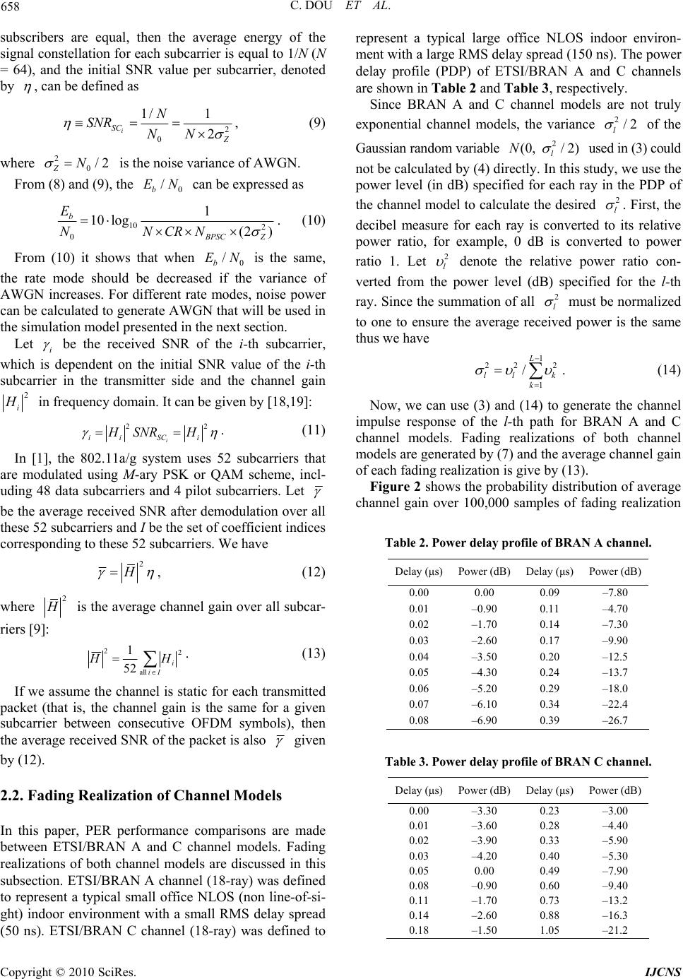

658 C. DOU ET AL.
subscribers are equal, then the average energy of the
signal constellation for each subcarrier is equal to 1/N (N
= 64), and the initial SNR value per subcarrier, denoted
by

, can be defined as
2
0
1/ 1
2
i
SC
Z
N
SNR NN 


, (9)
where is the noise variance of AWGN.
2
0/2
ZN
 
From (8) and (9), the can be expressed as
0
/
b
EN
10 2
0
1
10 log(2)
b
B
PSC Z
E
NNCRN

  . (10)
From (10) it shows that when is the same,
the rate mode should be decreased if the variance of
AWGN increases. For different rate modes, noise power
can be calculated to generate AWGN that will be used in
the simulation model presented in the next section.
0
/
b
EN
Let i

be the received SNR of the i-th subcarrier,
which is dependent on the initial SNR value of the i-th
subcarrier in the transmitter side and the channel gain
2
i
H
in frequency domain. It can be given by [18,19]:
2
i
iiSC i
HSNRH
2

 
. (11)
In [1], the 802.11a/g system uses 52 subcarriers that
are modulated using M-ary PSK or QAM scheme, incl-
uding 48 data subcarriers and 4 pilot subcarriers. Let

be the average received SNR after demodulation over all
these 52 subcarriers and I be the set of coefficient indices
corresponding to these 52 subcarriers. We have
2
H

 , (12)
where 2
H
is the average channel gain over all subcar-
riers [9]:



Ii
i
HH
all
2
2
52
1. (13)
If we assume the channel is static for each transmitted
packet (that is, the channel gain is the same for a given
subcarrier between consecutive OFDM symbols), then
the average received SNR of the packet is also

given
by (12).
2.2. Fading Realization of Channel Models
In this paper, PER performance comparisons are made
between ETSI/BRAN A and C channel models. Fading
realizations of both channel models are discussed in this
subsection. ETSI/BRAN A channel (18-ray) was defined
to represent a typical small office NLOS (non line-of-si-
ght) indoor environment with a small RMS delay spread
(50 ns). ETSI/BRAN C channel (18-ray) was defined to
represent a typical large office NLOS indoor environ-
ment with a large RMS delay spread (150 ns). The power
delay profile (PDP) of ETSI/BRAN A and C channels
are shown in Table 2 and Table 3, respectively.
Since BRAN A and C channel models are not truly
exponential channel models, the variance of the
Gaussian random variable used in (3) could
not be calculated by (4) directly. In this study, we use the
power level (in dB) specified for each ray in the PDP of
the channel model to calculate the desired
2/2
l

2
l
2
(0, /2)
l
N 

. First, the
decibel measure for each ray is converted to its relative
power ratio, for example, 0 dB is converted to power
ratio 1. Let 2
l

denote the relative power ratio con-
verted from the power level (dB) specified for the l-th
ray. Since the summation of all 2
l

must be normalized
to one to ensure the average received power is the same
thus we have
1
22
1
/
L
ll
k
2
k




. (14)
Now, we can use (3) and (14) to generate the channel
impulse response of the l-th path for BRAN A and C
channel models. Fading realizations of both channel
models are generated by (7) and the average channel gain
of each fading realization is give by (13).
Figure 2 shows the probability distribution of average
channel gain over 100,000 samples of fading realization
Table 2. Power delay profile of BRAN A channel.
Delay (μs)Power (dB)Delay (μs) Power (dB)
0.00 0.00 0.09 –7.80
0.01 –0.90 0.11 –4.70
0.02 –1.70 0.14 –7.30
0.03 –2.60 0.17 –9.90
0.04 –3.50 0.20 –12.5
0.05 –4.30 0.24 –13.7
0.06 –5.20 0.29 –18.0
0.07 –6.10 0.34 –22.4
0.08 –6.90 0.39 –26.7
Table 3. Power delay profile of BRAN C channel.
Delay (μs)Power (dB)Delay (μs) Power (dB)
0.00 –3.30 0.23 –3.00
0.01 –3.60 0.28 –4.40
0.02 –3.90 0.33 –5.90
0.03 –4.20 0.40 –5.30
0.05 0.00 0.49 –7.90
0.08 –0.90 0.60 –9.40
0.11 –1.70 0.73 –13.2
0.14 –2.60 0.88 –16.3
0.18 –1.50 1.05 –21.2

C. DOU ET AL.
659
for two channel models. A rectangle-based integration
method with equally spaced “bins” has been employed to
derive the curves. Here the width of each “bin” is 0.05.
From Figure 2, it shows that the mean value of both
probability distributions is equal to one. We see that for
small 2
H
, say smaller than 0.5, BRAN A channel has
higher probability distribution than that of BRAN C
channel. For instance, it gives 2 Pr( 0.5)H = 0.2316
for BRAN A channel and 2 Pr( 0.5)H = 0.0913 for
BRAN C channel. For large 2
H
, say larger than 2,
BRAN A channel also has higher probability distribution
than that of BRAN C channel. For instance, it gives
2
Pr( 2)H = 0.0788 for BRAN A channel and
2
Pr( 2)H = 0.0258 for BRAN C channel. The im-
pacts of 2
H
in its full statistics on the PER perform-
ance under BRAN A and C channel models are discussed
in the following.
Figure 3 shows the probability distribution of average
received SNR under two channel models given that the
rate mode RM = 3 and the target , denoted by T,
is 16 dB. Rectangle-based integration method with equ-
ally spaced “bins” has also been employed to derive the
probability distribution of average received SNR. For a
particular integer-valued average received SNR, R, the
range of the corresponding sampling bin is (R – 0.5, R +
0.5]. In this paper, only integer-valued average received
SNR is considered. However, fractionary average re-
ceived SNR can be treated by reducing the width of each
sampling bin. From (8) and (12), the average received
SNR of a packet for a certain rate mode can also be writ-
ten as
0
/
b
EN
2
10
10log()
B
PSC
HT CRN   (15)
Because of the code rate multiplied by the coded bits
per subcarrier is 1 for RM = 3, a simple relationship
2
H
T   holds in deriving the result of Figure 3. Al-
though the probability distribution of average received
SNR shown in Figure 3 has similarity to the probability
distribution of average channel gain shown in Figure 2,
Figure 3 depicts more clearly the influence of 2
H
on
average received SNR. The conclusions that have been
drawn from Figure 2 on the differences between BRAN
A and BRAN C channel models can be observed from
Figure 3 more apparently. In Figure 3, the pattern of the
probability distribution function defines the effective
range of average received SNR. The “effective” range
means that the probability distribution of average re-
ceived SNR falling outside of this range is negligible.
From Figure 3 we observe that the effective ranges of
average received SNR are different for two channel
models. The effective ranges are [7,22] dB and [10,21] dB
Figure 2. The probability distribution of average channel
gain over 100,000 samples of fading realization for BRAN A
and C channel models, respectively.
Figure 3. The probability distribution of average received
SNR in terms of average channel gain for two channel mod-
els given that RM = 3 and the target Eb/N0 is 16 dB.
for BRAN A and C channel models, respectively, for T =
16 dB. Clearly, BRAN A channel has longer tails on
both sides than BRAN C channel. Note that if the se-
lected rate mode and the target 0 are changed,
only the effective ranges of average received SNR are
shifted according to (15) but the patterns of the probabil-
ity distribution for both channel models remain un-
changed.
/
b
EN
2.3. PER Calculation for a Received Packet
The symbol error probability for an M-ary QAM [20]
with the average SNR per symbol, s, can be calculated
by
2
13
()111 erfc.
2( 1)
M
ps s
M
M




 












(16)

660 C. DOU ET AL.
In 802.11a/g, an OFDM data symbol consists of SD
N
= 48 data subcarriers. The average symbol error probabi-
lity for an M-ary QAM over all these data subcarriers can
be given by
,
1
1(),
SD
N
eMM i
i
SD
pp
N


 (17)
where i

is the received SNR of the i-th subcarrier. Wi-
th a Gray coding, the average bit error probability for an
M-ary QAM after demodulation is given by
,
2
1.
log
b
p
M
eM p (18)
In [21], an upper bound was given on the PER under
the assumption of binary convolutional coding and hard-
decision Viterbi decoding with independent errors into
the decoder. For a B-octet long packet to be transmitted
using PHY mode

, this bound is
8
,1(1),
B
epktu
pP

  (19)
where the union bound u
P

of the first-event error
probability is given by, free
ud
dd d
P
aP




 with
f
ree
d
being the minimum free distance of the convolutional
code for the given code rate, ad the total number of error
events of weight d [22], and Pd the probability of error in
the pair-wise comparison of two paths that differ in d bits.
When the hard-decision decoding is applied, Pd is given
by


 
12
2
2
21
1,
1
1,
2
2
ddk
k
bb
kd
d dd
ddk bb
k
bb
kd
dpp
k
dodd
Pdpp
dpp d
k
deven




 











 





(20)
where Pd is the average bit error probability given by (15).
2.4. Average PER of an Average Received SNR
For an B-octet long packet to be transmitted using rate
mode

, given that the target is T, total
100,000 samples of such packet are generated to derive
the average PER (an upper bound) of an average re-
ceived SNR by the following steps.
0
/
b
EN
Step 1: Calculate the initial SNR value per subcarrier
using (8).
Step 2: Calculate the average channel gain of each
sampling packet using (13).
Step 3: Calculate the average received SNR (

) of
each sampling packet using (12).
Step 4: Count the number of received packets, denoted
by , falling in the given sampling bin belonging
to the average received SNR R.
( )
pkt
NR
Step 5: Calculate the PER of each packet counted in
step 4 using (19).
Step 6: The average PER of the average received SNR
R, denoted by ()PERR, is given by
()
,
1
1
() []
()
pkt
NR
epkt
i
pkt
PER Rpi
NR
 (21)
where ,[]
epkt
p
i is the PER of the i- th packet calculated
in step 5.
2.5. Average PER Performance Comparisons
Figure 4 presents the performance comparisons of aver-
age PER derived in (21) between BRAN A and C chan-
nel models for four different rate modes defined in
802.11a/g, given that T = 16 dB and B is 196-octet long.
The effective range of average received SNR that can be
measured by (15) is considered for every PER curve of
different rate mode. For example, these ranges are [15,
30] dB and [18,29] dB for BRAN A and C channels, res-
pectively, given that RM = 8. From Figure 4 we observe
that BRAN C channel has better performance than BRAN
A channel for RM = 1 (6 Mb/s) and RM = 3 (12 Mb/s) if
the values of average received SNR are lower. On the
contrary, BRAN A channel outperforms BRAN C chan-
nel for RM = 6 (36 Mb/s) and RM = 8 (54 Mb/s) if the
values of average received SNR are higher. These results
agree with our observation from Figure 2 and Figure 3
Figure 4. Performance comparisons of average PER be-
tween BRAN A and C channels for four different rate
modes in 802.11a/g given that the target Eb/N0 is 16 dB.

C. DOU ET AL.
661
that BRAN A channel has higher probability to have
smaller values 2
H
than BRAN C channel. Thus, BR-
AN A channel degrades PER performance more severely
than BRAN C channel as channel conditions are bad.
Figure 2 and Figure 3 also show that BRAN A channel
has higher probability to have larger values of 2
H
than BRAN C channel. So that BRAN A channel out-
performs BRAN C channel on PER performance as
channel conditions are good.
The results and observations depicted above are rarely
found in the literature. Although many researchers have
focused on the performance evaluation of different cha-
nnel models in HiperLAN/2 and 802.11a, such as [12,23],
and it is commonly recognized that BRAN channel C has
better performance than channel A. For example, Haider
and Raweshidy in [23] concluded that BRAN C channel
has better performance than channel A due to the increa-
se of frequency diversity of the channels. Frequency di-
versity [24] due to delay spread provides the receiver
with several (ideally independent) replica of the trans-
mitted signal and is therefore a powerful means to com-
bat fading and interference. Surely BRAN C channel has
larger RMS delay spread (150 ns) than that of BRAN A
channel (50 ns). The ray (multipath) number of BRAN C
channel could be larger than that of BRAN A channel if
ideal exponential channel model was considered. But ac-
tually both channel models have the same ray number
(18-ray) and their PDPs are quite different as shown in
Table 2 and Table 3. In this paper, we provide a differ-
ent approach to compare the average PER performance
between two channel models. Our approach provides mo-
re insight into the performance differentiation between
BRAN A and BRAN C channel models by firstly taking
the whole power delay profiles of each channel model
into account, secondly by performing performance com-
parisons on a per target 0 basis, and thirdly by
considering the effects of the probability distribution of
average channel gain on the average PER performances.
Our approach for average PER performance comparisons
between different channel models can be applied to other
channel models as well, on a per target basis.
/
b
EN
0
/
b
EN
3. Simulation Model
Figure 5 shows the simulation model of OFDM-based
systems that we used in this paper. The inputs of the
simulation model are target , selected rate mode,
and packet length. The output of the simulation model is
the estimation of packet error rate. For a given target
and a certain selected rate mode, the initial SNR
value per subcarrier,
0
/
b
EN
0
/
b
EN

, is obtained by (8). Noise power
2
z

η
ˆi
H
Figure 5. The simulation model of OFDM-based systems.
is calculated by (10) to generate AWGN noise in the
simulation. In the IEEE 802.11a/g WLAN, there are two
long training symbols for each packet that can be used
for coherent detection. In this study training-sequence
based channel estimation method is used for stationary
mobile stations in slowly time-varying environments.
The two long training symbols in the PLCP (physical la-
yer convergence procedure) preamble are rate mode in-
dependent and are used for the channel estimation of
every received PPDU (physical protocol data unit). Other
channel estimation methods, such as pilot symbol aided
scheme [25-27], and blind estimation technique [28-30],
were not considered.
3.1. Channel Estimation
After taking an N point FFT at the receiver, the two long
training symbols have the same form of the received
signal for subcarrier i given by
[][], 0
niin
YiFH Zi n

 (22)
where {}
i
F
is the set of training sequence defined in
802.11a standard and is both known by the transmitter
and the receiver. In [31], a channel estimation value ˆi
H
of the i-th subcarrier in a conventional equalizer can be
estimated by
01
ˆ([] [])/2,
ii
H
Yi YiF (23)
where and are both complex Gaussian ran-
dom variables with the same mean
0[]Yi 1[]Yi
ii
H
F. In [32], it has
been proved that the optimal estimator of is just
i
H
ˆi
H
defined in (23) by using the likelihood function of
. The likelihood function of can be written as
i
Hi H

01
2
0
22
2
2
1
([][]; )
11
exp[([]
2/
2/
[])].
i
ii
Z
Z
ii
fYiYi H
Yi HF
N
N
Yi HF





 (24)

662 C. DOU ET AL.
The optimal estimator of is hence
i
H
01
2
01
01
ˆarg max ([][]; )
arg min [] []
([][])/2.
i
i
ii
H
ii ii
H
i
HfYiYiH
YiHFYi HF
Yi YiF



2
(25)
Thus, the estimation of the received SNR i

of the
ith subcarrier can be expressed as
2
ˆ
ˆ.
ii
H

  (26)
The estimation of the average channel gain over all
subcarriers is given by
22
all
1
ˆˆ.
52 i
iI
H

H
(27)
And the estimation of average received SNR of a
packet for a certain rate mode is given by
2
10
ˆ
ˆ10log().
BPSC
HT CRN   (28)
3.2. Analytical Upper Bound and Simulation
Results
In our simulation the size of the physical service data
unit (PSDU) is assumed 196-octet long. During transm-
ission, the PSDU is provided with a PLCP preamble and
header to create the PPDU. The simulation result of the
average PER for a particular average received SNR R is
obtained by first counting the number of those received
packets (PPDUs) whose estimated average received
SNRs falling within the range (R – 0.5, R + 0.5] but they
could not be decoded correctly, and then divided that nu-
mber by the value of defined in Subsection 2.4.
Figure 6 shows the results of average PER versus avera-
ge received SNR for three different values of target
under BRAN A channel model and RM = 7 (48 Mb/s).
The results of average PER derived both from the ana-
lytical upper bound and the simulation are presented for
comparison. From Figure 6, we can see that the results
derived from the analytical upper bound and derived
from the simulation can be fitted quite well for each case
of different target values, if the curve derived
from the analytical upper bound is shifted leftward by a
small amount less than 2 dB. The shifting amounts for T
= 22 dB, 19 dB and 16 dB are 2 dB, 1.8 dB and 1.5 dB,
respectively. A similar conclusion concerning the fitting
between PER curves derived from the analytical upper
bound and derived from the simulation in OFDM-based
systems can be found in [2].
()
pkt
NR
0
/
b
EN
/
b
E
0
N
In Figure 6, we also see that the PER curve of T = 16 dB
performs the best, and that of the T = 22 dB performs the
worst. This implies better PER performance is obtained
with the same average received SNR by lowering the
value of target . This phenomenon has close
relationship to the fading effects represented by
0
/
b
EN
2
H
, as
illustrated by the following example. For RM = 7, the
average received SNR value of a packet given by (20)
becomes 2
H
T   + 6 dB. For the case of T = 16 dB,
the average received SNR will be 25 dB if we let 2
H
= 2. The same average received SNR can be derived if
we let 2
H
= 1 and 2
H
= 1/2 for the cases of T = 19
dB and 22 dB, respectively. Though the average received
SNR for the above three cases are the same, the smallest
average PER is obtained by the case of T=16 dB under
better channel condition (2
H
= 2), and the largest ave-
rage PER is obtained by the case of T = 22 dB under
worse channel condition (2
H
= 1/2). The impact of
this phenomenon on the link adaptation of 802.11a will
be presented in the next section.
4. Numerical Results and Applications
For the rate adaptive 802.11a/g WLAN systems, this
section determines a set of mode switching thresholds for
each individual target using the results derived
above for the average PER, so that the optimal through-
put performance can be obtained on a per target
basis. The lower shifting of mode switching thresholds
with the lowering of target values is presented
by exploiting the phenomenon that we have observed
from Figure 6.
0
/
b
EN
b
E
0
/
b
EN
0
/N
Figure 6. Performance comparisons of average PER betw-
een the analytical upper bound and the simulation for three
different target Eb/N0 values under BRAN A channel mo-
del and RM = 7.

C. DOU ET AL.
663
ut-Based Link Adaptation
or throughput-based link adaptation, physical link is ad-
4.1. Throughp
F
apted to the rate mode that gives the highest throughput.
For different rate modes used in 802.11 a/g, the relation-
ship between the achieved throughput and the corresp-
onding average PER, denoted by PER , can be obtained
as follows. During transmission, SDU is provided
with a PLCP preamble and header to create the PPDU.
The transmission time of a PPDU frame (in us) can be
calculated as
PPDU
T
the P
(29)
where is the OFDM symbol interval, and
PREAMBLE SIGNAL
DATA_SYM SYM
T (16 us)T (4 us)
NT,


SYM
T
umbe
DATA_SYM
N
portion ofis the nr of OFDM symbols in the DATA
the PPDU frame format and its value is dependent on the
data rate used. The value of DATA_SYM N is calculated by
DATA_S YM
DBPS
16PSDU_size 86
N
,
N





(30)
where is the size of the PSDU in bytes, PSDU_size
DBPS is the nand Number of data bits per OFDM sym-
bol which is dependent on the rate mode used. To obtain
the net throughput of 802.11a/g physical layer, only the
payload bits of successful transmitted PPDU frames are
considered. Thus, the throughput (in Mb/s) is calculated
by
PPDU
Throughput=PSDU_size8(1) / T.PER (31)
We choose two target values
T = 12 dB
18
0
/
b
EN
oughpu
n unde
and
dB to illustrate the thrt-based link adaptation
of 802.11 a on a per target 0 /
b
EN basis. Average PER
derived from the simulatior BRAN A channel
model is used for all the cases presented in this section.
Both average PER and throughput versus average re-
ceived SNR for different rate modes under T = 12 dB and
18 dB are shown in Figure 7 and Figure 8, respectively.
Five contour lines for connecting points where 2
H
=
1/4, 1/2, 1, 2, and 4 on different average PER curveare
plotted in Figure 7(a). When compare Figure 7(a) to
Figure 8(a), firstly, we notice that contour lines with
smaller values of
s
2
H
which are absent in Figure 7(a)
are now appearingigure 8(a); secondly, the contour
lines that are of the same values of
in F2
H
are shifted
right toward higher average received SN Figure 8(a).
This is because for a particular rate mode to achieve a
certain average PER, the channel conditions, represented
by
R in
2
H
, experienced by the packets with lower target
EN is better than that experienced by the packets
her target 0 /
b
EN. For example, to achieve av-
erage PER = 10-2 fo 5 (24 Mb/s) in Figures 7(a)
and 8(a), the corresponding values of
0
/
b
with hig
r RM =2
H
are larger
than 2 for T = 12 dB and within [1/2, 1] fo= 18 dB. r T
(a)
(b)
Figure 7. Throughput-basedk adaptation for target Eb lin
0
/
N = 12 dB.
Figure 7(b) shows the throughput performances of
di
also means that there has no possibility to use RM = 1
fferent rate modes under T = 12 dB. Mode switching
between neighboring rate modes are clear except that
there has no definite rate adaptation between RM = 7 and
RM = 8. This exception is due to the right-most boundary
of the effective ranges of average received SNR for RM
= 7 and RM = 8 are 24 dB and 25 dB, respectively. In
Figure 7(b), the mode selection ranges for RM = 1 is [0,
7] dB, for RM = 3 is [8,13] dB, for RM = 5 is [14,18] dB,
for RM = 6 is [19,21] dB, for RM = 7 is [22,24], and for
RM = 8 is [25,-]. Figure 8(b) shows the result of link
adaptation for T = 18 dB. Simulation result shows that
there has no need for rate adaptation between RM = 3
(12 Mb/s) and RM = 1 (6 Mb/s). Therefore the through-
put curve for RM = 1 was not shown in Figure 8(b). This

664 C. DOU ET AL.
(a)
(b)
Figure 8. Throughput-basedk adaptation for target Eb
/N0 = 18 dB.
under BRAN A channel model. In Figure
(b), the mode selection ranges for RM = 3 is [9,13] dB,
Thresholds
s wved from Figure 6 that better PER
erformances with the same average received SNR are
ds with
lin
for T = 18 dB
8
for RM = 5 is [14,20] dB, for RM = 6 is [21,22] dB, for
RM = 7 is [23,27], and for RM = 8 is [28,31]. Note that
the effective ranges of average received SNR for differ-
ent rate modes are considered in both Figure 7 and Fig-
ure 8. Also in Figure 8, the two PHY rate modes RM = 2
(9 Mb/s) and RM = 4 (18 Mb/s) were not included. Be-
cause in our simulation, the throughput performance of
RM = 4 is worse than that of RM = 3 and the throughput
performance of RM = 2 is worse than that of RM = 1.
4.2. Lower Shifting of Mode Switching
e have obserA
p
obtained by lowering the values of target 0 /
b
EN. By
exploiting this phenomenon this subsection presents the
lower shifting of mode switching threshol the
lowering of target 0 /
b
EN values. An example is given
as below for illustrative purpose. Consider the results of
average PER for RM both Figures 7(a) and 8(a).
For RM = 7, we have already known that
= 7 in2
H
T   +
6 dB. For the case of T = 12 dB, the average received
SNR will be 21 dB if we let 2
H
= 2. Ther-
age received SNR is obtained if we let
e same av
2
H
= 1/2 for
the case of T = 18 dB. From Fe 7(a), we see that the
average PER of average received SNR = B is about
0.3 for RM = 7 under T = 12 dB. However, from Figure
8(a) we observe that this value is about 0.5 under T = 18
dB. Accordingly, the achieved net throughputs of aver-
age received SNR = 21 dB for RM = 7 are about 19 Mb/s
and 14 Mb/s under T = 12 dB and T = 18 dB, respec-
tively, as that shown in Figures 7(b) and 8(b). Therefore
we have shown that by lowering the value of T, better
throughput performance with the same average received
SNR can be achieved; consequently, rate adaptation to
the next lower rate mode can be shifted downwardly.
Compare the mode switching thresholds between RM = 6
and RM = 7 in Figures 7(b) and 8(b), we see that this
threshold is shifted downward from 22 dB under T = 18
dB to 21 dB under T = 12 dB.
Figure 9 provides a full view of the lower shifting of
mode switching thresholds fo
igur
21 d
r the link adaptation of
80
onding
An interesting phenomenon that can be observed from
2.11a over BRAN A channel model under different
target 0 /
b
EN values. In Figure 9, the X-axis denotes
the average received SNR and the Y-axis denotes the
desired ta0 /
b
EN. Six rate modes are considered in
the rate adaptation of 802.11a. The set of mode switching
thresholds for 0
/
b
EN = T dB can be obtained
from Figure 9 by drawing a horizontal line on T (Y-axis)
and finding the interseetween this horizontal line
and the vertical lines (mode switching boundaries). For
every given target 0 /
b
EN, the effective range of aver-
age received SNR is confined by the cross points plotted
on the both sides. Ts point on the right-hand side
is determined by the effective range of the highest rate
mode that the given target 0 /
b
EN may achieve; and
the cross point on the left-hand side is determined by the
effective range of the lowest rate mode that the given
target 0 /
b
EN may reach. Ideally, for every given value
of T there should have five mode switching thresholds
corresp to all the pairs of neighboring rate modes.
However, this may not be the case due to the rate modes
that can be adapted to under a specific value of T may
not cover all six rate modes. For example, the set of
mode switching thresholds under T = 18 dB is [-,13,20,
22,27] dB since there has no rate adaptation between RM
= 1 and RM = 3.
rget
target
ction
he cros
s b

C. DOU ET AL.
665
more frequently between neighboring
ra
this subsection, we show that no other sets of mode swi-
throughput
an the optimal set which is determined on a per target
22,27]
Figure 9 is that the lower shifting of mode switching thr-
esholds occurred
te modes RM = 7 and RM = 8 and also between RM = 5
and RM = 6. Coincidentally, each pair of neighboring
rate modes has the same and high modulation level. The
first pair, RM = 7 and RM = 8, uses the same modulation
scheme 64 QAM, and the second pair, RM = 5 and RM =
6, uses the same modulation scheme 16 QAM. The lower
shifting of mode switching thresholds occurred less freq-
uently between neighboring rate modes with different
modulation levels, for example RM = 3 with QPSK and
RM = 5 with 16 QAM. Moreover, there has no lower
shifting of mode switching thresholds between RM = 1
with BPSK and RM = 3 with QPSK. More investigations
are needed to further understand this phenomenon.
4.3. System Throughput Optimization
In
tching thresholds can achieve higher system
th
0
/
b
EN basis. The following example is given for illus-
trative purpose. From Figure 9, we have the optimal set
of mode switching thresholds under T = 18 dB is [-,13,20,
dB. Here we purposely choose two other sets of
mode switching thresholds [-,16,23,25,29] dB and [-,12,
18,20,24] dB. The thresholds in the first set are tending
towards right, so we called them upward-shifted thresh-
olds. On the contrary, the thresholds in the second set are
tending towards left, so we called them downward-shi-
fted thresholds. The comparisons of achieved system
throughputs between the optimal set and these two sets
of mode switching thresholds under T = 18 dB are pres-
ented in Figures 10(a) and 10(b), respectively. In Figure
10(a), the throughput achieved by the optimal set of mo-
de switching thresholds is expressed by the solid curves,
and that achieved by the upward-shifted thresholds is
expressed by the dotted curves. Obviously, the solid
curves are always higher than or equal to the dotted
curves for every average received SNR. In Figure 10(b)
we observe that rate adaptations using downward-shifted
thresholds always occurred at smaller average received
SNR values than that using the optimal thresholds. So
that solid curves are also higher than or equal to dotted
curves for every average received SNR in Figure 10(b).
5. Conclusions
Figure 9. A full view of the lower shifting of mode switching
thresholds for the link adaptation of 802.11a over BRAN A
channel model under different target Eb/N0 values.
ve 802.11a/g WLAN, an analytical
tain the average PER of indi-
For the rate adapti
pproach is proposed to oba
vidual average received SNR value for different rate mo-
des on a per target 0 /
b
EN basis. Instead of just looking
(a)
(b)
Figure 10. The comparisons of achieved system through
puts between the optimal set the other two sets of mode
switching thresholds: (a) Urd-shifted thresholds; (b)
-
and
pwa
Downward-shifted thresholds, under T = 18 dB.

C. DOU ET AL.
666
he National Science Coun-
racts NSC 96-2221-E
802.11a, Part 11: Wireless LAN Medium
l (MAC) and Physical Layer (PHY) Speci-
fications: High-speed Physical Layer in the 5GHz Band,
nsactions on Commu-
door
Proceedings of 4th International Con-
IEEE International
ystems,” Proceedings of IEEE Global Tele-
actions on Communications,
Commu-
ransactions on Mobile Computing, Vol. 1, No. 4,
oceedings of 56th IEEE Ve-
o Feedback Delay,” IEEE
a-
tion for OFDM,” Proceedings of IEEE In-
IEEE International Con-
at the average received SNR value of a packet, this paper
considers the whole distribution of the average received
SNR, which leads to a better average PER and through-
put performances. In this paper we also showed that the
probability distribution of average channel gain can af-
fect the average PER over the effective range of average
received SNR for different rate modes on a per target
0
/
b
EN basis. Furthermore, we have shown that better
PER performances with the same average received SNR
can bebtained by lowering the values of target 0
/
b
EN.
By exploiting this phenomenon, the mode switching
thresholds for optimal throughput performance of each
target 0
/
b
EN can be determined. Numerical results
show that mode switching thresholds can be shifted
downwh the lowering of target 0
/
b
EN values.
A full view of the lower shifting of mode switching
thresholds for the link adaptation of 802.11a over BRAN
A channel model under different target 0 /
b
EN values
is presented. From this an interesting phenomenon is
observed, that is, the lower shifting of mode switching
thresholds can occur more frequently between neighbor-
ing rate modes with the same and high modulation level
– e.g. 64 QAM or 16 QAM. The lower shifting of mode
switching thresholds occurred less frequently between
neighboring rate modes with different modulation levels
– e.g. QPSK and 16 QAM. Further investigations are
needed to have a better understanding of this phenome-
non.
6. Acknowledgements
o
ards wit
This work was supported by t
il, Taiwan, under the contc
0
-224- hicular Technology Conference, Vancouver, Vol. 2, 24-28
September 2002, pp. 738-742.
[13] L. B. Le, E. Hossain and M. Zorzi, “Queueing Analysis
for GBN and SR ARQ Protocols under Dynamic Radio
Link Adaptation with Non-Zer
02-MY2.
7. References
[1] IEEE Standard
Access Contro
Tran
Supplement to the IEEE 802.11 Standard, September 1999.
[2] O. Awoniyi and F. A. Tobagi, “Packet Error Rate in
OFDM-Based Wireless LANs Operating in Frequency
Selective Channels,” Proceedings of 25th IEEE Interna-
tional Conference on Computer Communications, Barce-
lona, 23-29 April 2006, pp. 1-13.
[3] J. Armstrong, “Analysis of New and Existing Methods of
Reducing Intercarrier Interference Due to Carrier Frequ-
ency Offset in OFDM,” IEEE Tra
nications, Vol. 47, No. 3, March 1999, pp. 365-369.
[4] W. Zhang and J. Lindner, “SINR Analysis for OFDMA
Systems with Carrier Frequency Offset,” Proceedings of
18th IEEE International Symposium on Personal, In
tern
and Mobile Radio Communications, Athens, 3-7 Septem-
ber 2007, pp. 1-5.
[5] Q. Yang, F. Fu, Y. Wu and K. S. Kwak, “Sub-Optimum
Superimposed Training Design for Estimating of Mobile
OFDM Channels,”
ference on Communications and Networking in China,
Xi’an, 26-28 August 2009, pp. 1-5.
[6] M. Lampe, H. Rohling and W. Zirwas, “Misunderstand-
ings about Link Adaptation for Frequency Selective Fad-
ing Channels,” Proceedings of 13th
Symposium on Personal, Indoor and Mobile Radio Com-
munications, Lisbon, Vol. 2, 15-18 September 2002, pp.
710-714.
[7] M. Lampe, T. Giebel, H. Rohling and W. Zirwas, “PER-
Prediction for PHY Mode Selection in OFDM Commu-
nication S
communications Conference, San Francisco, Vol. 1, 1-5
December 2003, pp. 25-29.
[8] C. Snow, L. Lampe and R. Schober, “Error Rate Analysis
for Coded Multicarrier Systems over Qusai-Static Fa-
ding Channels,” IEEE Trans
Vol. 55, No. 9, September 2007, pp. 1736-1746.
[9] H. Gong, W. Ye, S. Feng and H. Song, “A Subcarrier Al-
location Algorithm for Efficiently Reducing Power in
Multiuser OFDM Systems,” Wireless Personal
nications, Vol. 40, No. 2, 2007, pp. 233-243.
[10] J. Medbo and P. Schramm, “Channel Models for HIPE-
RLAN/2,” ETSI/BRAN Document Number 3ERI085B,
1998.
[11] D. Qiao, S. Choi and K. G. Shin, “Goodput Analysis and
Link Adaptation for IEEE 802.11a Wireless LANs,”
IEEE T
October 2002, pp. 278-292.
[12] S. Armour, A. Doufexi, A. Nix and D. Bull, “A Study of
the Impact of Frequency Selectivity on Link Adaptive
Wireless LAN Systems,” Pr
sactions on Wireless Communications, Vol. 6, No. 9,
September 2007, pp. 3418-3428.
[14] B. O’Hara and A. Petrick, “IEEE 802.11 Handbook–A
Designer’s Companion,” IEEE Press, Hoboken, 1999.
[15] M. R. Raghavendra, S. Bhashyam and K. Giridhar, “Fast
Multipath Delay Estimation in OFDM Systems Using
Frequency Swept Pilots,” Proceedings of 9th Intern
tional OFDM Workshop, Dresden, 15-16 September 2004,
pp. 237-240.
[16] N.-L. Hung, L.-N. Tho and C. C. Ko, “Joint Channel
Estimation and Synchronization with Inter-Carrier Inter-
ference Reduc
ational Conference on Communications, Glasgow, 24-
28 June 2007, pp. 2841-2846.
[17] J. Tao, J. Wu and C. Xiao, “Channel Estimation for OFDM
Systems in the Presence of Carrier Frequency Offset and
Phase Noise,” Proceedings of

C. DOU ET AL.
667
edings of IEEE International Conference
nsactions on Communications, Vol. 55,
ransactions on Commu-
ional Workshop on Mo-
ng Conference, Chi-
. 49, No. 12
ireless LANs for Mo-
M Systems Based on Pilots and
,” IEEE
eneralized Precoding,” IEEE
stimation for Cyclic Prefixed
ualization and Sampling Clock Tracking for
t Performance for the Rate
ference on Communications, Beijing, 19-23 May 2008,
pp. 5072-5076.
[18] H. Kang, W. Hwang and K. Kim, “OFDM Systems with
Subchannel Power Control under the Two-Ray Multipath
Channel,” Proce
on Communications, Helsinki, Vol. 6, 11-14 June 2001,
pp. 1856-1860.
[19] M. S. Bahaei, “Joint Optimization of Transmission Rate
and Outer-Loop SNR Target Adaptation over Fading Cha-
nnels,” IEEE Tra
No. 3, March 2007, pp. 398-403.
[20] S. Haykin, “Communication Systems,” 4th Edition, John
Wiley & Sons, Hoboken, 2001.
[21] M. B. Pursley and D. J. Taipale, “Error Probabilities for
Spread-Spectrum Packet Radio with Convolutional Codes
and Viterbi Decoding,” IEEE T
nications, Vol. 35, No. 1, January 1987, pp. 1-12.
[22] D. Haccoun and G. Begin, “High-Rate Punctured Con-
volutional Codes for Viterbi and Sequential Decoding,”
IEEE Transactions on Communications, Vol. 37, No. 11, MIMO OFDM Systems: Algorithm, Identifiability and
Performance Analysis,” IEEE Journal on Selected Areas
in Communications, Vol. 26, No. 2, February 2008, pp.
378-388.
[31] H.-W. Kim, C.-H. Lim and D.-S. Han, “Viterbi Decoder
Aided Eq
November 1989, pp. 1113-1125.
[23] K. Haider and H. S. Al-Raweshidy, “Evaluation of User
Capacity and Channel Model Effect in HiperLAN/2 Sys-
tem,” Proceedings of 4th Internat
bile and Wireless Communications Network, Stockholm,
9-11 September 2002, pp. 554-558.
[24] H. Bolcskei and A. J. Paulraj, “Space-Frequency Coded
Broadband OFDM Systems,” Proceedings of IEEE Wire-
less Communications and Networki
cago, Vol. 1, 23-28 September 2000, pp. 1-6.
[25] M. Morelli and U. Mengali, “A Comparison of Pilot-
Aided Channel Estimation Methods for OFDM Systems,”
IEEE Transactions on Signal Processing, Vol,
Ada
December 2001, pp. 3065-3073.
[26] R. Gruenheid, H. Rohling, J. Ran, E. Bolinth and R. Kern,
“Robust Channel Estimation in W
bile Environments,” Proceedings of 56th IEEE Vehicular
Technology Conference, Vancouver, Vol. 3, 24-28 Septem-
ber 2002, pp. 1545-1549.
[27] Z. Yuanjin, “A Novel Channel Estimation and Tracking
Method for Wireless OFD
Kalman Filtering,” IEEE Transactions on Consumer Elec-
tronics, Vol. 49, No. 2, May 2003, pp. 275-283.
[28] A. P. Petropulu, R. Zhang and R. Lin, “Blind OFDM Cha-
nnel Estimation through Simple Linear Precoding
Transactions on Wireless Communications, Vol. 3, No. 2,
March 2004, pp. 647-655.
[29] F. Gao and A. Nallanathan, “Blind Channel Estimation
for OFDM Systems via G
Transactions on Vehicular Technology, Vol. 56, No. 3,
May 2007, pp. 1155-1164.
[30] F. Gao, Y. Zeng, A. Nallanathan and T. S. Ng, “Robust
Subspace Blind Channel E
OFDM WLAN,” Proceedings of 60th IEEE Vehicular
Technology Conference, Los Angeles, Vol. 5, 26-29 Sep-
tember 2004, pp. 3738-3742.
[32] W.-C. Liu, L.-C. Wang and Y.-W. Lin, “Physical Layer
Effects on the MAC Goodpu
ptive IEEE 802.11a/g WLAN,” Proceedings of IEEE
Wireless Communications and Networking Conference,
Atlanta, Vol. 3, 21-25 March 2004, pp. 1873-1878.