Journal of Global Positioning Systems (2004)
Vol. 3, No. 1-2: 70-78
Analysis of Biases Influencing Successful Rover Positioning with
GNSS-Network RTK
Hans-Jürgen Euler
Leica Geosystems AG, Heinrich-Wild-Strasse, CH-9435 Heerbrugg (Switzerland)
e-mail: [e-mail]; Tel: [phone]: Fax: [phone]
Stephan Seeger
Leica Geosystems AG, Heinrich-Wild-Strasse, CH-9435 Heerbrugg (Switzerland)
e-mail: [e-mail]; Tel: [phone]; Fax: [phone]
Frank Takac
Leica Geosystems AG, Heinrich-Wild-Strasse, CH-9435 Heerbrugg (Switzerland)
e-mail: [e-mail]; Tel:[phone] ; Fax: [phone]
Received: 15 November 2004 / Accepted: 16 February 2005
Abstract. Using the Master-Auxiliary concept, described
in Euler et al. (2001), Euler and Zebhauser (2003)
investigated the feasibility and benefits of standardized
network corrections for rover applications. The analysis,
focused primarily in the measurement domain,
demonstrated that double difference phase errors could be
significantly reduced using standardized network
corrections. Extended research investigated the potential
of standardized network RTK messages for rover
applications in the position domain (Euler et al, 2004-I).
The results of baseline processing demonstrated effective,
reliable and homogeneous ambiguity resolution
performance for long baselines (>50km) and short
observation periods (>45 sec). In general horizontal and
vertical position accuracy also improved with the use of
network corrections. This paper concentrates on the
impact of wrongly determined integers within the
reference station network on RTK performance. A
theoretical study using an idealized network of reference
stations is complemented by an empirical analysis of
adding incorrect L1 and L2 ambiguities to the
observations of a real network. In addition, the benefits of
using network RTK corrections for a small sized network
in Asia during a period of high ionospheric activity is
also demonstrated.
Key words: Master-Auxiliary concept, dispersive errors,
non-dispersive errors, approximation, influence of wrong
ambiguities.
1 Introduction
Standardization of RTCM SC104 network RTK messages
is still in progress. In the absence of a standard, this paper
uses the Master-Auxiliary concept (MAC) as described in
Euler et al. (2001) to analyse the effect of various biases
on network RTK positioning performance. MAC closely
resembles the format adopted by the RTCM working
group as the basis for network RTK messages.
MAC uses so-called dispersive and non-dispersive phase
correction differences to compress network RTK
information without the need for standardized correction
models. To understand how MAC compresses this
information consider the single difference L1 phase
equation j
km 1,
∆Φ for stations k (the reference) and m (the
auxiliary) and a satellite j.
1 1,
1
2
1
1, 1,
)(
)(
)()()()(
ε
δ
∆+∆⋅+
∆
−∆+
∆⋅+∆+∆=∆Φ
j
km
j
km
j
km
km
j
km
j
km
j
km
N
f
c
f
tI
tT
tdtctrtst
(1)
where
j
km
s∆ geometric range term including antenna phase
centre variations which have been applied by the
network processing software.
j
km
r δ ∆ broadcast orbit error.
km
dt
∆
receiver clock error.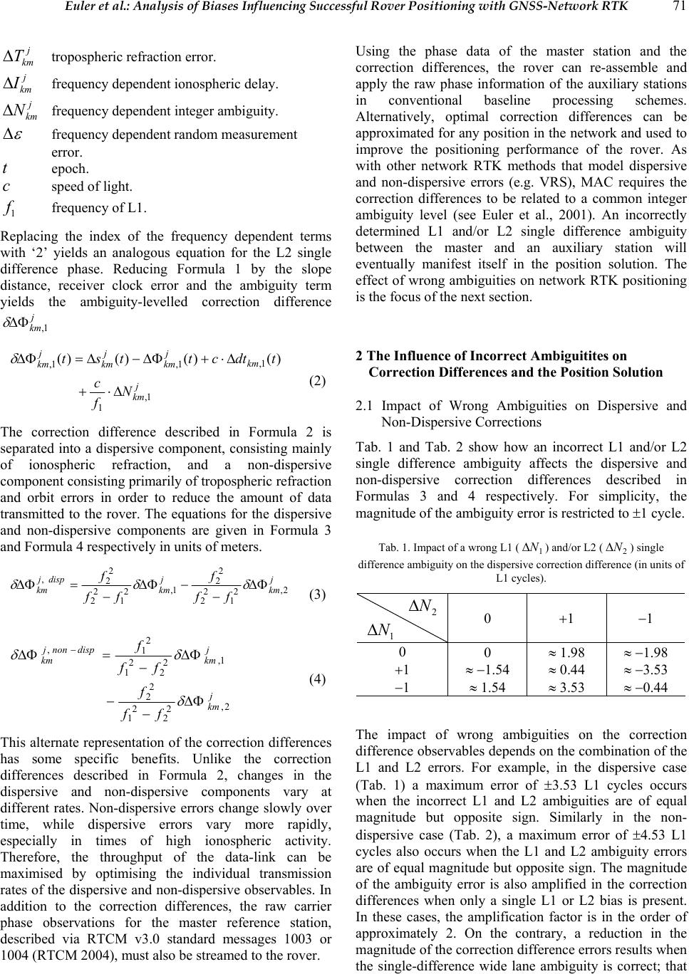

Euler et al.: Analysis of Biases Influencing Successful Rover Positioning with GNSS-Network RTK 71
j
km
T∆ tropospheric refraction error.
j
km
I∆ frequency dependent ionospheric delay.
j
km
N∆ frequency dependent integer ambiguity.
ε
∆ frequency dependent random measurement
error.
t epoch.
c speed of light.
1
f frequency of L1.
Replacing the index of the frequency dependent terms
with ‘2’ yields an analogous equation for the L2 single
difference phase. Reducing Formula 1 by the slope
distance, receiver clock error and the ambiguity term
yields the ambiguity-levelled correction difference
j
km 1,
∆Φ δ
j
km
km
j
km
j
km
j
km
N
f
c
tdtcttst
1,
1
1, 1,1, )()()()(
∆⋅+
∆⋅+∆Φ−∆=∆Φ δ
(2)
The correction difference described in Formula 2 is
separated into a dispersive component, consisting mainly
of ionospheric refraction, and a non-dispersive
component consisting primarily of tropospheric refraction
and orbit errors in order to reduce the amount of data
transmitted to the rover. The equations for the dispersive
and non-dispersive components are given in Formula 3
and Formula 4 respectively in units of meters.
j
km
j
km
dispj
km ff
f
ff
f
2,
2
1
2
2
2
2
1,
2
1
2
2
2
2
,∆Φ
−
−∆Φ
−
=∆Φ δδδ
(3)
j
km
j
km
dispnonj
km
ff
f
ff
f
2,
2
2
2
1
2
2
1,
2
2
2
1
2
1
,
∆Φ
−
−
∆Φ
−
=∆Φ −
δ
δδ
(4)
This alternate representation of the correction differences
has some specific benefits. Unlike the correction
differences described in Formula 2, changes in the
dispersive and non-dispersive components vary at
different rates. Non-dispersive errors change slowly over
time, while dispersive errors vary more rapidly,
especially in times of high ionospheric activity.
Therefore, the throughput of the data-link can be
maximised by optimising the individual transmission
rates of the dispersive and non-dispersive observables. In
addition to the correction differences, the raw carrier
phase observations for the master reference station,
described via RTCM v3.0 standard messages 1003 or
1004 (RTCM 2004), must also be streamed to the rover.
Using the phase data of the master station and the
correction differences, the rover can re-assemble and
apply the raw phase information of the auxiliary stations
in conventional baseline processing schemes.
Alternatively, optimal correction differences can be
approximated for any position in the network and used to
improve the positioning performance of the rover. As
with other network RTK methods that model dispersive
and non-dispersive errors (e.g. VRS), MAC requires the
correction differences to be related to a common integer
ambiguity level (see Euler et al., 2001). An incorrectly
determined L1 and/or L2 single difference ambiguity
between the master and an auxiliary station will
eventually manifest itself in the position solution. The
effect of wrong ambiguities on network RTK positioning
is the focus of the next section.
2 The Influence of Incorrect Ambiguitites on
Correction Differences and the Position Solution
2.1 Impact of Wrong Ambiguities on Dispersive and
Non-Dispersive Corrections
Tab. 1 and Tab. 2 show how an incorrect L1 and/or L2
single difference ambiguity affects the dispersive and
non-dispersive correction differences described in
Formulas 3 and 4 respectively. For simplicity, the
magnitude of the ambiguity error is restricted to ±1 cycle.
Tab. 1. Impact of a wrong L1 (1
N∆) and/or L2 (2 N∆) single
difference ambiguity on the dispersive correction difference (in units of
L1 cycles).
2
N
∆
1
N
∆
0 +1 −1
0 0 ≈ 1.98 ≈ −1.98
+1 ≈ −1.54 ≈ 0.44 ≈ −3.53
−1 ≈ 1.54 ≈ 3.53 ≈ −0.44
The impact of wrong ambiguities on the correction
difference observables depends on the combination of the
L1 and L2 errors. For example, in the dispersive case
(Tab. 1) a maximum error of ±3.53 L1 cycles occurs
when the incorrect L1 and L2 ambiguities are of equal
magnitude but opposite sign. Similarly in the non-
dispersive case (Tab. 2), a maximum error of ±4.53 L1
cycles also occurs when the L1 and L2 ambiguity errors
are of equal magnitude but opposite sign. The magnitude
of the ambiguity error is also amplified in the correction
differences when only a single L1 or L2 bias is present.
In these cases, the amplification factor is in the order of
approximately 2. On the contrary, a reduction in the
magnitude of the correction difference errors results when
the single-difference wide lane ambiguity is correct; that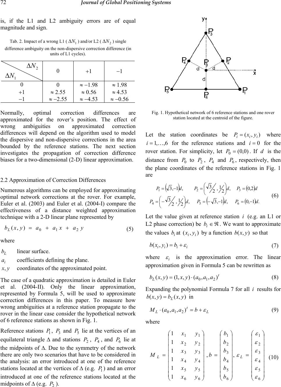

72 Journal of Global Positioning Systems
is, if the L1 and L2 ambiguity errors are of equal
magnitude and sign.
Tab. 2. Impact of a wrong L1 (1 N∆) and/or L2 (2 N∆) single
difference ambiguity on the non-dispersive correction difference (in
units of L1 cycles).
2
N∆
1
N∆ 0 +1 −1
0 0 ≈ −1.98 ≈ 1.98
+1 ≈ 2.55 ≈ 0.56 ≈ 4.53
−1 ≈ −2.55 ≈ −4.53 ≈ −0.56
Normally, optimal correction differences are
approximated for the rover’s position. The effect of
wrong ambiguities on approximated correction
differences will depend on the algorithm used to model
the dispersive and non-dispersive corrections in the area
bounded by the reference stations. The next section
investigates the propagation of correction difference
biases for a two-dimensional (2-D) linear approximation.
2.2 Approximation of Correction Differences
Numerous algorithms can be employed for approximating
optimal network corrections at the rover. For example,
Euler et al. (2003) and Euler et al. (2004-I) compare the
effectiveness of a distance weighted approximation
technique with a 2-D linear plane represented by
yaxaayxb L210 ),( ++= (5)
where
L
b linear surface.
i
a coefficients defining the plane.
y
x
, coordinates of the approximated point.
The case of a quadratic approximation is detailed in Euler
et al. (2004-II). Only the linear approximation,
represented by Formula 5, will be used to approximate
correction differences in this paper. To measure how
wrong ambiguities at a reference station propagate to the
rover in the linear case consider the hypothetical network
of 6 reference stations as shown in Fig. 1.
Reference stations 1 P, 3 P and 5 P lie at the vertices of an
equilateral triangle ∆ and stations 2 P, 4 P, and 6 P lie at
the midpoints of ∆. Due to the symmetry of the network
there are only two scenarios that have to be considered in
the analysis: an error introduced at one of the reference
stations located at the vertices of ∆ (e.g. 1 P) and an error
introduced at one of the reference stations located at the
midpoints of ∆ (e.g. 2 P).
Fig. 1. Hypothetical network of 6 reference stations and one rover
station located at the centroid of the figure.
Let the station coordinates be ),(iii yxP = where
6,,1 …
=
i for the reference stations and 0=i for the
rover station. For simplicity, let )0,0(
0=P. If d is the
distance from 0 P to 2 P, 4 P and 6 P, respectively, then
the plane coordinates of the reference stations in Fig. 1
are
(
) ()
() () .1,0,1,3,
2
1
,
2
3
2,0,
2
1
,
2
3
,1,3
654
321
dPdPdP
dPdPdP
−=−−=





−=
=






=−= (6)
Let the value given at reference station i (e.g. an L1 or
L2 phase correction) be ℜ
∈
i
b. We want to approximate
the values i bat ),(ii yx by a function ),(yxb so that
iiiibyxb
ε
+
=
),( (7)
where i
ε
is the approximation error. The linear
approximation given in Formula 5 can be rewritten as
t
Laaayxyxb ),,(),,1(),( 210
⋅= (8)
Expanding the polynomial Formula 7 for all i results for
),(),( yxbyxb L
=
in
L
t
LbaaaM
ε +=⋅ ),,( 210 (9)
where




















=




















=




















=
6
5
4
3
2
1
6
5
4
3
2
1
66
55
44
33
22
11
,,
1
1
1
1
1
1
ε
ε
ε
ε
ε
ε
ε
LL
b
b
b
b
b
b
b
yx
yx
yx
yx
yx
yx
M
(10)

Euler et al.: Analysis of Biases Influencing Successful Rover Positioning with GNSS-Network RTK 73
The polynomial coefficients t
Laaaa),,( 210
≡ that
minimize 2
L
ε
are given by
() bMMMa t
LL
t
LL
1 −
=. (11)
Substituting ),( ii yx from Formula 6 into L M yields the
following expression for
()
t
LL
t
LMMM 1−:
()
















−−−
−−=
−
dddddd
dddd
MMM t
LL
t
L
15
2
15
2
15
1
15
4
15
1
15
2
0
15
32
15
3
0
15
3
15
32
6
1
6
1
6
1
6
1
6
1
6
1
1
(12)
Assume that the values i b differ from the correct values
i
b by i b∆, i.e. iii bbb∆+= . Substituting
t
bbbbbb ),,(6611 ∆+∆+=∆+ … into Formula 11 leads
to a natural splitting of the polynomial coefficients L a
into terms L abelonging to band terms a∆belonging to
b∆.
() ()
LL
t
LL
t
LL
aa
bbMMMa
∆+=
∆+= −
!
1
(13)
where
() bMMMat
LL
t
LL
1−
= and
() bMMMa t
LL
t
LL ∆=∆−1.
(14)
Thus, following from Formula 8 the change in the
approximated value at ),(yxP= due to the reference
station biases b∆ is given by
LL ayxyxb∆⋅=∆ ),,1(),( (15)
The analysis is restricted to the following two cases:
Case 1: error
δ
introduced at 1 P,
i.e. t
b)0,0,0,0,0,( δ =∆
Case 2: error
δ
introduced 2 P,
i.e. t b)0,0,0,0,,0( δ =∆ .
Substituting b
∆
for case 1 and case 2 into Formula 14
yields together with Formula 15 the following general
expressions for the change in the approximated value
at ),(yxP
=
:
Case 1: () δ
t
Ldd
yxyxb 






−⋅=∆ 15
2
,
15
32
,
6
1
,,1),(
(16)
Case 2: () δ
t
Ldd
yxyxb 







⋅=∆ 15
1
,
15
3
,
6
1
,,1),( (17)
For the rover station )0,0(
0
=
P, located at the centre of
the network, Formulas 16 and 17 reduce to the following
simplified expressions
Case 1: δ
6
1
)0,0( =∆ L b
Case 2: δ
6
1
)0,0( =∆ L b
In fact further analysis, which has been omitted from the
text for the sake of brevity, using additional reference
stations placed on a circle around the rover shows that the
linear approximation attenuates the introduced error by a
factor of about n1 where nis the number of stations
used in the network.
More generally, Fig. 2 illustrates the magnitude of the
approximated error for any station),( yxP = with
1
=
=
δ
d.
Note that the approximated error is largest in the vicinity
of the biased station. More accurately, the magnitude of
the error depends on the distance of the approximated
station from the biased reference station along the line of
maximum gradient. The closer the approximated station
is, the larger the error.
The preceding theoretical study demonstrates the
propagation of reference station biases for the linear
approximation; however, it does not measure the impact
of these biases on the network RTK performance. To
complement the theoretical study, the following section
empirically investigates the actual impact of wrong
ambiguities on the final position solution.

74 Journal of Global Positioning Systems
Fig. 2. Case 1: the approximated error at a station ),(yxP = resulting
from a bias at one of the reference stations 1 P, 3 P or 5 P.
2.3 Impact Of Incorrect Ambiguities On The Position
Solution.
For the empirical analysis, four hours of 1 Hz dual-
frequency data was collected on the network of 4 stations
depicted in Fig. 3, which form part of the SAPOS
permanent reference station network in Bavaria,
Germany.
33 km
81 km
61 km
100000.0 m100000.0 m
271
270
258
269
Master
Auxiliary
Rover
Fig. 3. Distribution of reference stations in the test network. Station 258
was the designated master and station 271 was used to simulate the
rover.
The double-difference phase ambiguities between the
reference stations 258, 269 and 270 were determined and
dispersive and non-dispersive corrections differences,
described by Formulas 3 and 4 respectively, were
computed using station 258 as the master. Optimal
network corrections were approximated for the rover
station (271) and subsequently applied to the data. The 2-
D linear approximation given by Formula 5 was used for
the interpolation process. The corrected data was then
processed using discrete observation times of 60 seconds.
All the solutions were fixed correctly; a fixed solution
being deemed correct if the difference of the height
component to the true height of the rover station was less
than ±5 cm.
In the first experiment, a bias of +1 cycle was added to
the L2 ambiguity of satellite 6 at station 270 before
computing the dispersive and non-dispersive correction
differences. The L2 frequency was chosen to simulate the
real-world situation where the fixing and keeping of L2
ambiguities is generally more problematic compared to
L1. Since L2 has no civil code and the P-code is
encrypted, proprietary tracking techniques are used to
recover the range and phase information. This process
yields L2 observables with a higher relative noise and
causes the phase measurement to be more susceptible to
cycle-slips than L1 at low elevations. Using the biased
data, optimal network corrections were computed and the
observations reprocessed as previously described. Fig. 4
shows the fixed solutions for the observation period in
relation to the elevation of the biased satellite and time.
Correctly fixed solutions are shown as solid green
squares while solutions with incorrectly fixed ambiguities
are represented as hollow red squares.
Sat6 L2(+1) on 270
10
20
30
40
50
60
70
80
90
15:00:00 15:30:00 16:00:00 16:30:0017:00:00 17: 30:0 0 18: 00 :00 18:30:00
observation time (hh:mm:ss)
el
ev
ati
on
Fig. 4. The number of fixed solutions using corrected data. A bias of +1
cycle was added to the L2 ambiguity of satellite 6 at station 270 before
computing the correction differences. Correctly fixed solutions are
shown as solid green squares and incorrectly fixed solutions are
represented as hollow red squares.
Ambiguity resolution was generally problematic
especially when the biased satellite was above an
elevation of 60 degrees. The problem to fix ambiguities
was expected since an incorrect L2 or L1 ambiguity is
amplified in the dispersive and non-dispersive correction
differences by a factor of almost 2 (see Section 2.1).
According to Tab. 1 and Tab. 2, one could expect fewer
problems fixing if both the L1 and L2 ambiguities were
biased so that the widelane ambiguity is still valid, since
the influence of this bias is reduced by a factor of
approximately 2 in the respective correction differences.
To test this hypothesis, biases of +1 cycle were added to
the L1 and L2 ambiguities of satellite 6 at station 270
prior to generating the correction differences. Optimal
correction differences were then applied at the rover and
the data reprocessed. The results are depicted in Fig. 5.

Euler et al.: Analysis of Biases Influencing Successful Rover Positioning with GNSS-Network RTK 75
Sat6 L1(+1) L2(+1) on 270
10
20
30
40
50
60
70
80
90
15:00:00 15:30 :0 0 16:00 : 0 0 16: 30 :00 17:00:00 17:30:00 18: 00 :0 0 18:30:00
observation time (hh:mm:ss)
el
ev
ati
on
Fig. 5. The number of fixed solutions using corrected observations.
Biases of +1 cycles were added to the L1 and L2 ambiguities of satellite
6 at station 270 prior to computing the correction differences.
Ambiguity resolution is still problematic when the biased
satellite is above an elevation of 60 degrees. However,
below this elevation the ambiguity resolution
performance has improved. There are more correctly
fixed solutions and importantly the number of wrongly
fixed solutions has decreased by approximately 1/2. One
could expect further improvement in the fixing
performance if the biased station was further from the
rover due to the distance dependency inherent in the
linear interpolation algorithm (see Section 2.2). Station
269 is approximately twice the distance from the rover as
station 270. Biases of +1 cycle were added to the L1 and
L2 ambiguities of satellite 6 at this station instead of 270
and the data processed as before.
Sat6 L1(+1) L2(+1) on 269
10
20
30
40
50
60
70
80
90
15:00:00 15:30:0 0 16:00 : 0 0 16:30: 0 0 17:00:00 17: 30:00 18: 00 : 0 0 18:30 : 0 0
observation time (hh:mm:ss)
ele
va
tio
n
Fig. 6. The number of fixed solutions using corrected observations.
Biases of +1 cycles were added to the L1 and L2 ambiguities of satellite
6 at station 269 prior to computing the correction differences.
Again, successful ambiguity resolution is still
problematic above 60 degrees. However, below this
elevation there are more correctly fixed solutions
compared to the results of the previous test (Fig. 5),
especially in the elevation band between 25 and 40
degrees. These results also highlight a trait common to
the previous two tests; the impact of wrong ambiguities
on the position solution is less when the bias is present on
a low elevation satellite. To test this premise, a bias of +1
cycle was added to the L2 ambiguity of satellite 10 at
station 269. Satellite 10 reached its highest elevation of
approximately 20 degrees midway through the
observation period. Optimal correction differences were
computed for the rover as usual and the data processed
for the interval when satellite 10 was above the elevation
cut-off. The fixed solutions are shown in Fig. 7.
Sat10 L2(+1) on 269
10
20
30
40
50
60
70
80
90
15:00:00 15:30:00 16:00:00 16:30:00 17:00:00 17:30 :0 0 18: 00 :0 0 18:30 :0 0
observation time (hh:mm:ss)
ele
v
a
t
io
n
Fig. 7. A bias of +1 cycle was added to the L2 ambiguity of satellite 10
at station 269.
In comparison to the results of the first experiment,
described in Fig. 4, the biased satellite has a minimal
impact on ambiguity resolution performance; although, it
should be noted that a few solutions were fixed
incorrectly. For completeness, biases of +1 cycle were
added to the L1 and L2 ambiguities of satellite 10 at
station 269 and the data reprocessed. The results are
given in Fig. 8.
Sat10 L1(+1) L2(+1)on 269
10
20
30
40
50
60
70
80
90
15:00:00 15:30:00 16:00:00 16:30:00 17:00:00 17:30 :0 0 18: 00 :0 0 18:30 :0 0
observation time (hh:mm:ss)
ele
v
a
t
io
n
Fig. 8. The number of fixed solutions using corrected observations.
Biases of +1 cycle were added to the L1 and L2 corrections of this
satellite at station 269.
As expected, when the wide lane ambiguity is correct the
biased satellite has virtually no impact on ambiguity
resolution performance. In order to analyse the effect of
biases on low elevation satellites in more detail, the
dispersive and non-dispersive errors for the master-rover
baseline (258-271) were grouped into elevation bins of 1
degree according to the elevation of the lowest satellite
used to build the double difference. For each elevation
bin, the average and mean true errors were calculated
where the mean true error is given by:
n
][ εε
ε = (18)
and
ε
is the true error and n is the number of
observations. The graph of the average and mean true
dispersive errors for the unbiased data is shown in Fig. 9.

76 Journal of Global Positioning Systems
GF 271-258 cor
-0.3
-0.2
-0.1
0
0.1
0.2
0.3
0.4
0 20 40 60 80
elevation
cy
cle
s average
true error
Fig. 9. Corrected average and mean true dispersive errors for the
baseline 271-258.
The dispersive errors are generally less than 0.1 cycles
and apparently random as indicated by the average error
line. In addition, the magnitude of the errors decreases
linearly with increasing elevation as shown by the mean
true error line. For comparison, the average and mean
true dispersive errors are also shown when the bias of +1
cycle was added to the L2 ambiguity of satellite 10 at
station 269.
GF Sat10 L2(+1)271-258 c
-0.3
-0.2
-0.1
0
0.1
0.2
0.3
0.4
0 20 40 60 80
elevation
cy
cle
s average
true error
Fig. 10. Corrected average and true dispersive errors for the baseline
271-258. A bias of +1 cycle was added to the L2 ambiguities of satellite
10 at station 269.
As expected, only the dispersive errors below an
elevation of 20 degrees are affected. In this elevation
band, a bias of approximately +0.1 cycles has been added
to the dispersive errors. Combined with an elevation
dependent observation weighting strategy, which is
common to many baseline processing algorithms, the
effect of this bias on the position solution is further
reduced. Conversely, the observations of high elevation
satellites are given a higher weight by the processor and
have a greater influence on the position solution. The
problem can be compounded for if the biased high
elevation satellite happens to be chosen as the reference.
Consider the following average and mean true dispersive
errors for the same baseline with an L2 ambiguity bias of
+1 cycle added to the observations of the reference
satellite 21.
The resulting dispersive errors are biased by
approximately +0.3 cycles across virtually all elevations.
This bias is larger by a factor of 3 compared to the
previous example for the low elevation satellite. By itself,
this bias will have a negative impact on ambiguity
resolution and when coupled with an elevation dependent
weighting strategy effective high-precision positioning
can be severely hampered.
GF Sat21 L2(+1)271-258 c
-0.4
-0.3
-0.2
-0.1
0
0.1
0.2
0.3
0.4
020 40 60 80
elevation
cy
cle
s
average
true error
Fig. 11. Corrected average and mean true dispersive errors for the
baseline 271-258. A bias of +1 cycle was added to the L2 ambiguities of
the reference satellite 21 at station 269.
Several conclusions can be drawn from the empirical
analysis presented in this section. First, the influence of
wrongly fixed ambiguities on the position solution is
greater for high elevation satellites. The problem can be
compounded if the reference satellite ambiguity has been
fixed incorrectly. Second, the influence of a wrongly
fixed reference station ambiguity on positioning
performance at the rover is distance dependent. The
closer the rover is to the reference station, the larger the
effect. However, this conclusion is heavily dependent on
the approximation algorithm used to derive optimal
network corrections for the rover station. Thirdly, the
influence of a wrongly fixed wide lane ambiguity is less
than a single L1 or L2 ambiguity bias. The strength of
these conclusions should be considered together with the
fact that the results can be heavily influenced by satellite-
station geometry and the choice of the approximation and
processing algorithms employed. In addition, several
other biases can have a negative impact on positioning
performance, high ionospheric activity for example,
which is the subject of the following section.
2 Analysis of the Effect of high Ionosphere on
Network RTK
For a network of 6 stations located in Hong Kong, 4
hours of 1 Hz data were collected on the 14th November
2003 between 04:00 am and 08:00 am during a period of
known high ionospheric activity (IPS Radio and Space
Services, 2003). According to the data archive of the
Center for Orbit Determination in Europe (CODE) at the
Astronomical Institute of the University of Berne, the
TEC (Total Electron Content) value at the respective
location and time was about 450. For comparison, the
TEC value at the same time for the mid of Germany was
about 44. The stations of the network are depicted in
Fig. 12.

Euler et al.: Analysis of Biases Influencing Successful Rover Positioning with GNSS-Network RTK 77
Cycle slips were removed from the raw data prior to the
estimation of the double-differenced phase ambiguities
between the reference stations. The resulting ambiguity-
levelled data was used to form dispersive and non-
dispersive correction differences. Station HKSL
represents the master reference station. The remaining
stations serve as auxiliaries, except for station HKKT,
which is the designated rover. The length of the master-
rover baseline is 16.4km. The closest reference station to
the rover is HKLT approximately 7.8km away. This
baseline, being the shortest, would be used in a usual
baseline algorithm where no network corrections were
applied and therefore serves as a reference for analysing
the benefit of using approximated corrections.
The percentages of fixed ambiguities resulting from
different processing strategies on the shortest baseline
and also for the master-rover baseline are listed in Tab. 3.
These percentages were used as the measure of
processing performance.
Master
A
uxiliar
y
Rover
20000.0 m
HKSL
HKLT
HKKT
HKFN
HKST
HKSC
9.2 km
13.3 km
15.6 km
7.8 km
16.4 km
Master
A
uxiliar
y
Rover
Master
A
uxiliar
y
Rover
20000.0 m
HKSL
HKLT
HKKT
HKFN
HKST
HKSC
HKSL
HKLT
HKKT
HKFN
HKST
HKSC
9.2 km
13.3 km
15.6 km
7.8 km
16.4 km
Fig. 12. Distribution of auxiliary reference stations in relation to the
rover station HKKT. Station HKSL was the designated master reference
station.
Tab. 3. Percentage of fixed ambiguities for the shortest baseline in the Hong Kong network and for the baseline between rover and master for
different processing strategies.
Baseline Processing Mode Percentage of Fixed Ambiguities
HKKT - HKLT No corrections, no stochastic modelling 17.5
HKKT - HKSL No corrections, ionospheric activity low 32.8
HKKT - HKSL No corrections, ionospheric activity medium 76.9
HKKT - HKSL Applied corrections (D=1, ND=15), no stochastic modelling 97.2
HKKT - HKSL Applied corrections (D=1, no ND), no stochastic modelling 94.4
HKKT - HKSL Applied corrections (D=1, ND=1), no stochastic modelling 100
HKKT - HKSL Applied corrections, (D=1, no ND), ionospheric activity low 100
D=x, ND=y determine the update rates in seconds for
dispersive (D) and non-dispersive (ND) corrections. In all
cases an observation time of 45 seconds and an elevation
mask of 10 degrees was chosen.
RTK systems are usually tuned for most general
observing conditions. Users should not be required to
change special processing parameters, especially when
they have no indication when and what to change.
Therefore, baselines shorter than 10 km are usually
processed in real-time without stochastically modelling
the ionosphere (in order not to confuse multipath or
obstructions with ionospheric noise). For this reason no
stochastic modelling was used on the shortest baseline
HKKT – HKLT. Baselines between 10 and 20 km are
already in the range where ionospheric biases are more
likely to be present and affect positioning results. For
such baselines, real-time algorithms would stochastically
model the ionosphere using parameters associated with a
low ionospheric activity setting. In post-processing, an
operator might check which ionospheric setting produces
the optimal solution, as demonstrated in Tab. 3 where the
low and medium ionospheric activity settings were tested
for the short baseline. However, this approach is not
feasible in real-time since the system deals with short
occupation times and has no indication of long-time
behaviour. To compare the effectiveness of network
corrections with a usual approach, the master-rover
baseline was processed with the standard ionospheric
settings that would be used if no corrections were
applied.
As described in the introduction, the update rates of the
dispersive and non-dispersive corrections are chosen
differently to maximise the data throughput. For this
experiment, an update rate of 1 Hz was always used for
the dispersive errors. For the non-dispersive errors an
update rate of 15 seconds was compared with an update
rate of 1 second. In addition, the effect of applying
dispersive but no non-dispersive corrections (D=1,no
ND) was also tested. The percentage of fixed solutions
increases from 17.5% on the shortest baseline HKKT –
HKLT to 97.2% on the rover-master baseline HKKT –
HKSL when an update rate of 15 seconds for the non-
dispersive corrections (which is a typical update rate for a
real-world application) was used. Increasing the update
rate for the non-dispersive errors to 1 Hz increases the
number of fix solutions to 100%. It should be emphasized
that these results are achieved without stochastic
modelling. When the ionospheric activity setting for
ionospheric stochastic modelling is set to low, 100%

78 Journal of Global Positioning Systems
fixed solutions are also obtained without any non-
dispersive corrections. These results compare favourably
to the 32.8% of fixed solutions obtained on the short
baseline when no network corrections were applied. This
analysis illustrates the benefits of using network
corrections in the presence of relatively high ionospheric
disturbances even for a small sized network.
3 Conclusions
The effect of various combinations of wrong L1 and L2
integers on the correction difference observables, which
could be introduced by either wrong initial fixing or
undetected cycle slips, was tabulated and the propagation
of these biases in a 2-D linear approximation was
analysed for an idealized network of reference stations.
The actual impact on ambiguity resolution was
investigated by comparing unbiased results with
computations where artificial ambiguities were added to
the observations. The processing results showed that a
bias on only one frequency affects the final performance
of a real-time system more than when the widelane is still
valid; that is when identical biases for both frequencies
are present. Therefore, correction differences with a
correct widelane ambiguity, which are provided for in the
current RTCM SC104 network RTK message proposal,
could help to fix the ambiguities of low elevation
satellites. These observations may eventually have to be
down-weighted.
Reference station networking is usually considered as an
approach for achieving better RTK performance over
long baseline lengths. It is often argued that establishing a
reference station network with inter-station distances of
only a couple of 10kms is excessive. However the
example of the Hong Kong network, with an average
reference station separation of less than 15km, shows that
ionospheric disturbances can be severe in equatorial
regions and hamper effective positioning on baselines
usually considered as unproblematic. The additional
information provided by surrounding reference stations
increased the performance of RTK positioning from very
unfavourable, with only 32.8% fixed solutions, to high
performance with a success rate of 100%.
Acknowledgements. We thank Mr. Andreas Brünner of
SAPOS Bayern for kindly supplying us the Bavarian data
set and Mr. Simon Kwok of the Geodetic Surveying
Section, Hong Kong Lands Department for the Hong
Kong data set.
References
CODE data archive, ftp://ftp.unibe.ch/aiub/CODE/
Euler, H.-J., Keenan, C.R., Zebhauser, B. E., Wübbena, G.
(2001) Study of a Simplified Approach in Utilizing
Information from Permanent Reference Station Arrays,
ION GPS 2001, September 11-14, 2001, Salt Lake City,
UT
Euler, H.-J., Zebhauser, B. E., Townsend, B., Wübbena, G.
(2002) Comparison of Different Proposals for Reference
Station Network Information Distribution Formats, ION
GPS 2002, September 24-27, 2002, Portland, OR
Euler, H.-J., Zebhauser, B.E. (2003) The Use of Standardized
Network RTK Messages in Rover Applications for
Surveying, ION NTM 2003, January 22-24, 2003,
Anaheim, CA
Euler, H.-J., Seeger, S., Zelzer, O., Takac, F., Zebhauser, B. E.
(2004-I) Improvement of Positioning Performance Using
Standardized Network RTK Messages, ION NTM 2004,
January 26-28, 2004, San Diego, CA
Euler, H.-J., Seeger, S., Takac, F. (2004-II) Influence of
Diverse Biases on Network RTK, ION GNSS 2004, Long
Beach, CA
RTCM (2004) RTCM Recommended Standards for
Differential GNSS (Global Navigation Satellite Systems)
Service, Version 3.0, RTCM paper 30-2004-SC104-STD.
Zebhauser, B. E., Euler, H.-J., Keenan, C.R., Wübbena, G.
(2002) A Novel Approach for the Use of Information
from Reference Station Networks Conforming to RTCM
V2.3 and Future V3.0, ION NTM 2002, January 28-30,
2002, San Diego, CA.