ABSTRACT

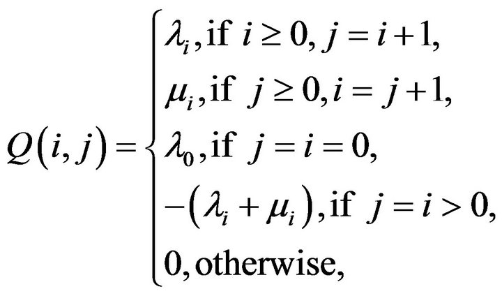
Let Q be the Q-matrixof an irreducible, positive recurrent Markov process on a countable state space. We show that, under a number of conditions, the stationary distributions of the n × n north-west corner augmentations of Q converge in total variation to the stationary distribution of the process. Twoconditions guaranteeing such convergence include exponential ergodicity and stochastic monotonicity of the process. The same also holds for processes dominated by a stochastically monotone Markov process. In addition, we shall show that finite perturbations of stochastically monotone processes may be viewed as being dominated by a stochastically monotone process, thus extending the scope of these results to a larger class of processes. Consequently, the augmentation method provides an attractive, intuitive method for approximating the stationary distributions of a large class of Markov processes on countably infinite state spaces from a finite amount of known information.

1. Introduction

Let 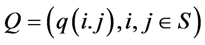be the stable, conservative of a continuous-time Markov process on a countable state space The satisfies

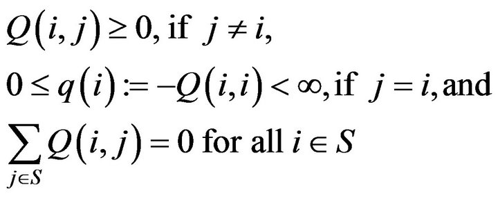
In addition, we assume that Q is regular, which means there exists no non-trivial, non-negative solution

to

for some (and then all).

Under these assumptions, the state transition probabilities of the process are given by the unique Q-function which satisfies the Kolmogorov backward equations,

The object, which is also called a transition function, is a family of matrices indexed over the reals which constitutes an analytic semi-group. an analytic semi-group is characterised by three properties: is the identity matrix, the row sums of are less than or equal to unity and is equal to the matrix product for all. This last property, known as the Chapman-Kolmogorov equation, implies. Thus, even though F^t is generally thought of as the matrix of state transition probabilities at time t, it serves as an analogue to the t-th power of the transition matrix of a discrete-time Markov chain on the state space Consequently, using the superscript to denoteas a function of t should not cause any confusion. While on the subject of notation, we should mention that we are using a standard notation common in the literature of continuous-time Markov processes on general state spaces. In the discrete state space setting, this notation causes matrices to look like functions of two variables (or kernels) while measures and vectores appear to be functions over the state space. We have elected to follow this notation in an endeavour to reduce the number of subscripts and superscripts in the sequel.

Note that in the conservative setting posed here, regularity of is equivalent to honesty and uniqueness of the transition function, that is, for all

The state space is irreducible if for all. On such a state space, a Markov process is said to be positive recurrent or ergodic if for all as. For a positive recurrent process, it can be shown (for example, see Theorem 5.1.6 in [1]) that the satisfies

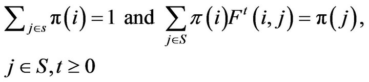(1)

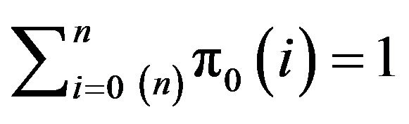
More generally, any measure satisfying (1) is called an invariant or stationary measure for the process. If, in addition, the measure has mass 1, it is referred to as a stationary or invariant distribution. Any measure satisfying (1) with “” replaced by “” is called a subinvariant measure for. Conversely, if F has a stationary distribution, then the process is positive recurrent and.

In this paper, we are interested in approximating using the north-west corner truncations of. The analogous problem for discrete-time Markov chains has been studied in [2-7]. The final reference contains a review of the literature on the discrete-time version of the truncation problem. Some properties of truncation in continuous-time Markov processes were studied in [8,9].

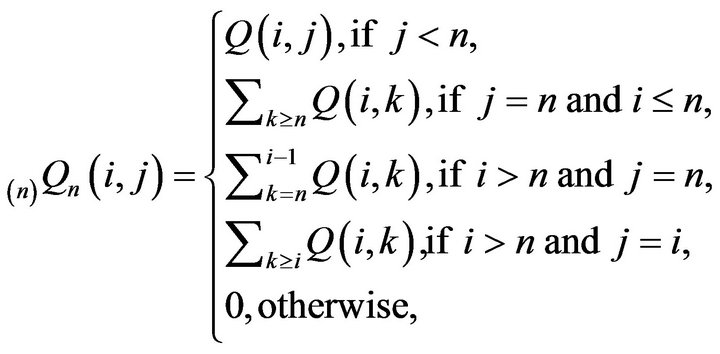
Truncations of Q are submatrices of Q defined by

, where

and is an increasing sequence of subsets of S such that.

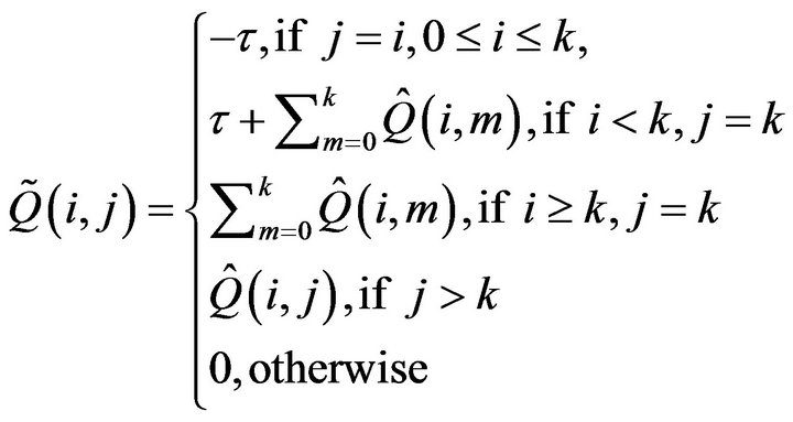
The truncation is not conservative. By adding the discarded transition rates to, we may produce a conservative which generates a uniquehonest, finite, continuous-time Markov process. For example, we may choose to perform linear augmentation, where the aggregate of the transition rates outside of is dispersed amongst the states in according to some probability measure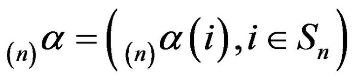. Then, the

order augmentation is given by

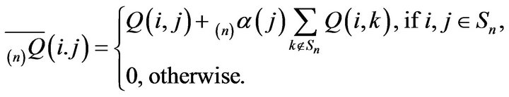
An important example of this is where we only augment a single column, say, in which case is the Dirac measure at h and we obtain The order augmentation as

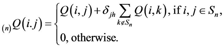
Here, 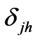denotes the kronecker delta.

Linear augmentation obtains exactly one irreducible, closed class together with zero or more open classes from which A_n is accessible. Since is closed,

is conservative on and so the minimal

is honest and positive recurrent on

. Finiteness of ensures that the remaining open classes are transient. Hence, there exists a unique invariant measure for. We shall be mainly concerned with where either or. The minimal will be denoted while

will be its invariant probability measure.

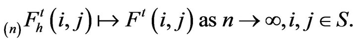
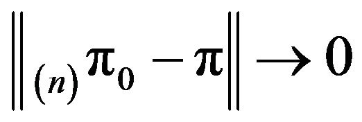
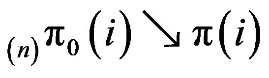
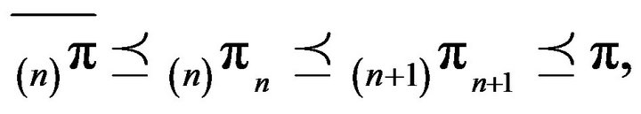
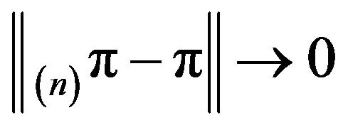
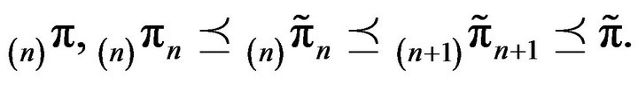
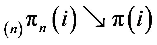
Two obvious questions now arise. Firstly, when does

(2)

Here, we use to denote convergence in total variation norm. Secondly, how quickly does this convergence occur? This paper considers the first question. We shall present augmentation strategies for approximating invariant distributions for two classes of Markov processes via for n large. The classes are:

• Markov processes which satisfy

for some. Such processes are called exponentially ergodic.

• Stochastically monotone Markov processes, which have the property that

for all, and processes dominated by stochastically monotone processes.

Parallelling results for discrete-time chains in [7], we shall also show that Markov processes constructed from finite perturbations of stochastically monotone processes are always dominated by some other stochastically monotone process. This extends the class of processes for which our results are applicable.

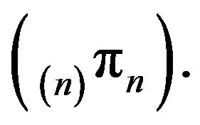
In the next section, we begin by showing that the limit of the is unique when it exists. Then, Section 3 considers exponentially ergodic Markov processes while Section 4 studies stochastically monotone Markov processes and their above-mentioned variations.

Finally, some concluding remarks are made in Section 5.

2. Preliminaries

The problem of proving that may be broken into two parts. Firstly we must show that converges weakly to some limit, say, and secondly, that. We consider the latter in this section.

Theorem 2.1 Consider a sequence of linearly augmented derived from Q and let

be the minimal -function. Then

(3)

Proof: Let denote the minimal -function.

Firstly, observe that 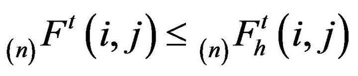for all

and. This can be seen inductively using the backward integral recurrences for and. The argument parallels the proof of Theorem 2.2.14 in [1] which states that

(4)

for all

Next, since is honest and is dishonest, we see that

(5)

for, where

(6)

Applying (4) to (6) together with monotone convergence shows that monotonically decreases to 0 as. Taking limits in n on both sides of (5) then completes the proof.

Remark 2.2 Although we have only considered linear augmentations, the statement and proof of Theorem 2.1 is in fact valid for any sequence of augmentations

.

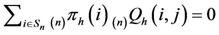
Since the transition function is finite, it is positive recurrent on some subset of. Hence it possesses a unique stationary distribution and

(7)

for. Positive recurrence establishes anequivalence between the stationary distributions for and invariant distributions for. An invariant distribution for an arbitrary is any probability measure such that 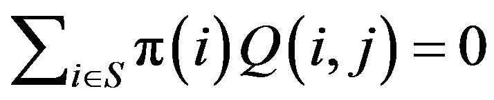for all

. So, uniquely satisfies

for all

Let us assume for the moment that converges weakly to some limit measure. We require that. Weak convergence to implies that is a probability distribution. By taking the limit infimum on both sides of (7) and applying Fatou’s Lemma, we have

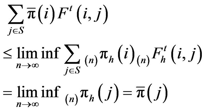
for. The measure is therefore a subinvariant probability measure for. However, is positive recurrent and hence, by Theorem 4 in [10], is both invariant and the unique probability measure satisfying (1). Hence,.

3. Exponential Ergodicity

Let Q be the of a positive recurrent Markov process on. Consider an increasing sequence of sets such that and

for all n. Let be the truncation of corresponding to. In this section, we shall consider augmentations obtained by linearly augmenting in column 0. We shall prove that exponential ergodicity of the Markov process is sufficient for as where is taken to be, the invariant distribution for. In order to do this, we shall require the notion of a -norm. Let be an arbitrary vector (function) such that for all. In future, we abreviate this to. The - norm of a signed measure n is then

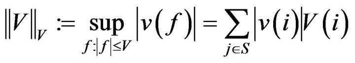
If 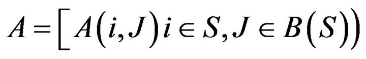is a matrix, then the -norm of is

Rather than working with the Q-matrix augmentationsdirectly, we will use the -resolvents associated with these. The -resolvent of a continuoust-time Markov process is the stochastic matrix

given by,

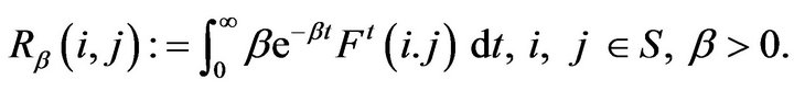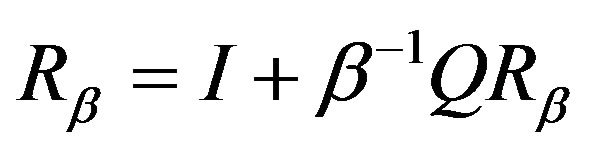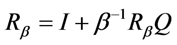We note that satisfies the resolvent forms of both the backward and forward equations which are and respectively.

Since is regular, is the unique solution to the resolvent form of the backward equations. Let and denote the unique -resolvents of and respectively. Here, is the minimal -funcction while denotes the minimal - function. Since is a finite set, , and have the same invariant distribution. The same is true for and, which share the distribution.

In the sequel, we shall have need of the following corollary to Theorem 2.1.

Corollary 3.1

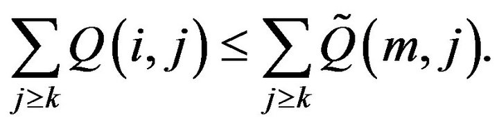
i. For all,

(8)

where; and ii..

Proof: Part i is obtained by integrating both sides of (5) with respect to be. Part ii then follows by taking limits in (8) and observing that

and as

Next, the various “drift to C” conditions introduced in [11] will play an important role in allowing us to pass between the continuous-time process and the discretetime -resolvent chain. The drift conditions require the notion of a petite set in both continuoustime processes and discrete-time chains. Let denote the Borel -algebra on S. Then, A set is a petite set in the continuous-time setting if there exists a probability distribution on and a non-trivial positive measure such that

for, where.

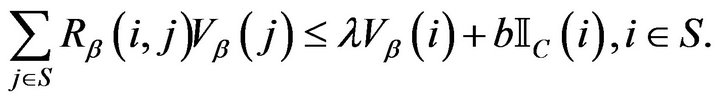
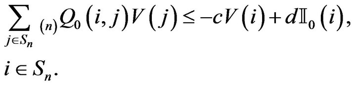
Petite sets for discrete-time chains are defined analogously. According to Theorem 5.1 in [11], the following three drift conditions are equivalent, although the petite set C and function V may differ in each instance.

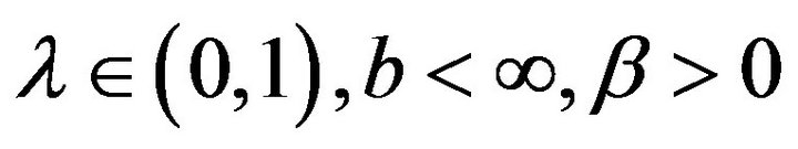
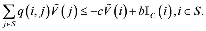
: Drift for T-skeletons. For some, there exist constants bounded for all with, together with a petite set and a function such that

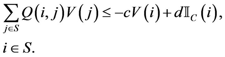
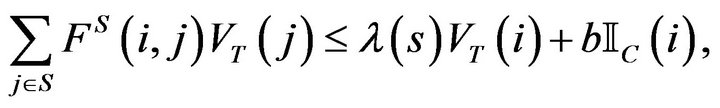
for. We use to denote the indicator function of the set C which is 1 if and 0 otherwise.

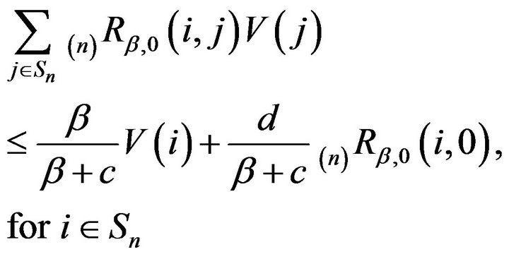
: Drift for -resolvents. For some

, a petite set and a function

: Drift for the Q-matrix. For constants a petite set and a function

An irreducible continuous-time Markov process X is -uniformly ergodic if, for some invariant probability kernel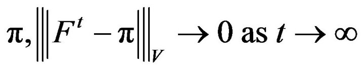. In the special case where, the chain is said to be uniformly ergodic or strongly ergodic: For all as

where, by an abuse of notation, we use to denote the invariant transition kervnel for all

The following theorem collects together a number of results on exponential and -uniform ergodicity of Markov processes from the literature.

Theorem 3.2 Let X be an irreducible, aperiodic continuous-time Markov process on S. The following conditions are equivalent.

i. One of the drift conditions holds, in which case they all hold, but not necessarily with the same petite set;

ii. For all, the T-skeleton chain is geometrically ergodic;

iii. For all, the -resolvent chain is geometrically ergodic;

iv. X is exponentially ergodic.

v. X is -uniformly ergodic for some.

In particular, it is -uniformly ergodic, -uniformly ergodic and -uniformly ergodic where and satisfy respectively.

Proof:

iiiiiiv. This was proved in Theorem 5.3 of [11].

iiv. Theorem 5.1 of [11] shows that

satisfy a solidarity property in that either all of them hold or none hold. Next, fix and set which is trivialy petite Since it is finite. In, set and, where

and the’s are those appearing in Theorem 3 of [12]. Finally, an appropriate relabelling of the states in

reveals to be equivalent to the necessary and sufficient condition for exponential ergodicity givenin Part (ii) of Theorem 3 in [12]. Consequently X is exponentially ergodic if and only if orany of the other drift criteria holds.

iv. Theorem 5.2 in [11] says that any of is sufficient for X to be -uniformly ergodic where is either or respectively.

vii. If X is-uniformly ergodic for some, then so to is the - skeleton for any and an application of Theorem 16.0.1 in [13] shows that

for some and.

Geometric ergodicity of the -skeleton then follows from the definition of the -norm.

Next, suppose that the Markov process X is exponenttially ergodic. From Theorem 3.2, there exist constants and a function such that

(9)

Without loss of generality, we may take and assume that. The state space can always be relabelled to accommodate this convention. Then, since for all, the augmented -matrices each satisfy

Multiplying both sides by and re-arranging, we obtain

.

Now, choose 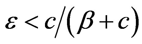such that

for some

. This is always possible since is a strictly positive matrix (in particular, and, as noted in the proof of Corollary 3.1,

as. Therefore,

. So, in addition to

being strongly aperiodic, we see that is strongly aperiodic for all. A transition matrix is strongly aperiodic if it is primative and possesses a non-zero diagonal entry.

Define. By Proposition 5.5.4 in [13], the set is petite since the singleton set is trivially petite and is uniformly accessible from under the resolvent chain, that is,

is bounded away from 0 for all. By the definition of, we have for

. On the other hand, 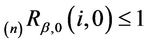for

, since is a stochastic matrix. Hence we have

(10)

(11)

where and.

Note that for all large enough.

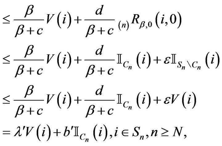
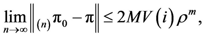
Next, set 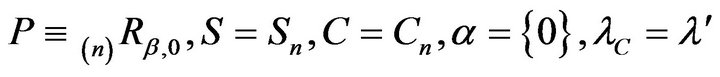and in Theorem 6.1 of [14]. It can be seen that the conditions of the theorem are satisfied and so there exists some such that

where 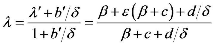and

. Furthermore, we have

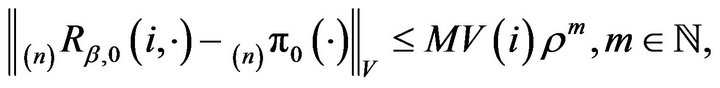
where is the unique invariant distribution for, and and are completely determined by and. Note that this is true for every so that the rate of convergence is independent of the truncation size. In addition, by applying the preceding argument directly toinstead of, we also have for all m, sinceby assumption, (9) holds and. Thus, not only are and V-uniformly ergodic, they are geometrically ergodic with the same convergence rate.

We can now prove the main result of this section.

Theorem 3.3 Let X be an exponentially ergodic, continuous-time Markov chain on a countable, irreducible state space. Let and be the invariant distributions for and respectively. Then,

as.

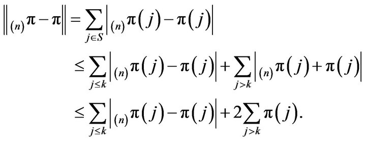
Proof: Choose an arbitrary number. From the triangle inequality, we have

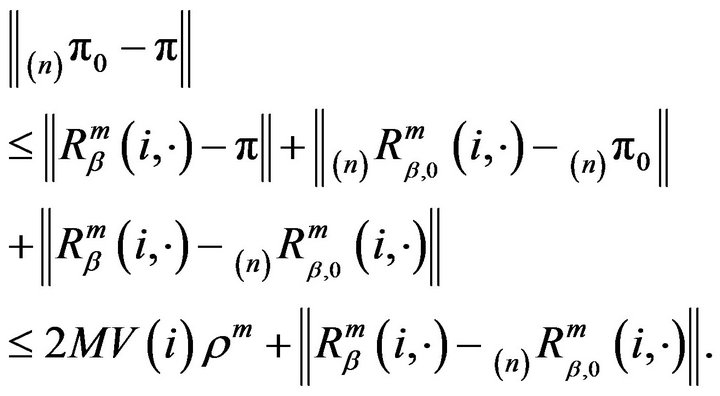(13)

As was pointed out in [7], if and are two stochastic matrices, then

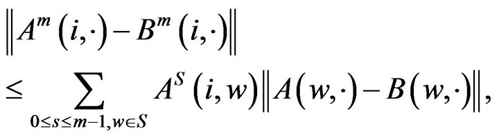(14)

for. Applying this to the last term in (13), we obtain

(15)

where

Now, since as for all, we can use dominated convergence to conclude that the third term in (13) vanishes as n tends to infinity. Thus,

for, and since m was chosen arbitrarily,

.

Example

Let and define by

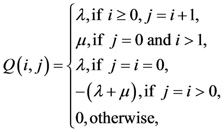
The process with this -matrix is essentially a renewal process with renewal times marked by visits to state 0. Each renewal time consists of a geometric number of exponential times of mean followed by an exponential time of mean. At each jump, the process passes from stateto statewith probability and falls back to state 0 with probability. the state space is clearly irreducible and the process has a geometric stationary distribution, where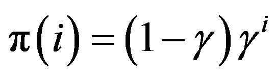. Existence of the stationary distribution ensures positive recurrence.

Next, let the vector be given by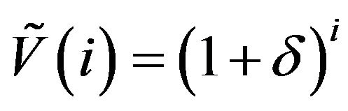, where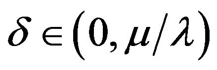. Also define and Set

, where c is a small positive number. Then, the drift condition holds for the specified and. The process is therefore exponentially ergodic by Theorem 3.2. Further, all the conditions of Theorem 3.3 are satisfied. Thus, we can construct augmentations on corresponding sets 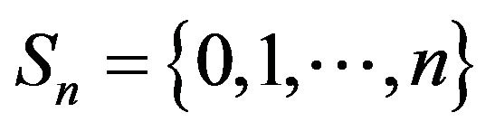and use their invariant distributions to approximate.

We can confirm this by solving

with

. We have

for, from which it is evident that

(as. Convergence in total variation follows by the same argument used later in the proof of Theorem 4.2.

4. Stochastic Monotonicity

In this section, we develop results for stochastically monotone Markov processes. Our key result says that stochastic monotonicity of the process is sufficient for (2) to hold under arbitrary linear augmentation. The remaining results extend this to larger classes of Markov processes. While our methods generally parallel those employed in [6] TO study the same problem in discrete-time Markov chains, itt is necessary to take greater care constructing the augmentations in the continuous-time setting.

Let and be two non-trivial measures. Then,

stochastically dominates if

for all, in which case we write. If and are two transition functions, we say that stochastically dominates (written) if, for all  for all A more strict classification is stochastic comparability. The transition functions and are stochastically comparable if for all and with We use the notation to mean that and are stochastically comparable. A stochastically monotone Markov process is one whose transition function is stochastically comparable to itself. Thus, if is stochastically dominated by a transition function which itself is stochastically monotone, then and are stochasticallly comparable. Clearly, implies

The following theorem is the key to obtaining sufficient conditions for (2) to hold in continuous time. It characterises stochastic comparability and monotonicity in terms of-matrix structure and is a special case of a more general result which was proved in [15] (also see Theorem 7.3.4 in [1] for an account). The reader is directed to the last two citations for the proof.

Theorem 4.1 ([15] and [1, Chapter 7.3])

i. Let and be two conservative -matrices. Their corresponding minimal transition functions and are stochastically comparable iff, whenever and k is such that either or then

(16)

ii. Let be a conservative -matrix. Its minimal -function F is stochastically monotone iff, Whenever and k is such that either or then

(17)

As a consequence of this result, we shall speak of stochastically monotone Q-matrices and of two Q-matrices as being stochastically comparable, etc. This abuse of terminology should not cause any confusion.

If is an irreducible, positive recurrent transition function and it stochastically dominates another irreducible transition function then is also positive recurrent. Furthermore, if and denote the stationary distributions of F and respectively, then which can be seen by letting in

In fact, we may say something stronger than this. If is reducible and contains a collection of closed ireducible classes each C_i is positive recurrent with invariant probability measure Since F is dominated by on it follows that Now, any invariant measure on for can be written as a linear combination of the’s; that is, for some probability measure Therefore, for all invariant distributions.

Throughout the rest of this section, we shall use the north-west corner truncations of that is, truncations of the form for

4.1. Stochastically Monotone Processes

Let be the -matrix of a positive recurrent, stochastically monotone Markov process F. By construction, the north-west corner truncations of augmented in the nth column are stochastically monotone. Since is conservative on a finite set  has precisely one positive recurrent class, which contains and is a subset of or equal to Its limiting distribution satisfies

for all From Theorem 4.1, we also see that is stochastically monotone.

Let be an arbitrary augmentation of and note that is stochastically comparable with As per our comments above, the minimal -function is positive recurrent on one or more irreducible subsets of and hence any invariant distribution for

, say is stochastically dominated by

Now, let us extend and to S as follows:

(18)

and

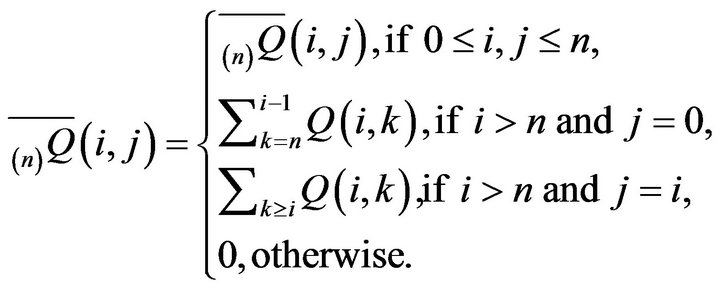
We also extend and to by appending a countably infinite number of 0’s to each, so that for all Note that

(resp.) remains invariant for (resp.).

Moreover, since the minimal -function is positive recurrent on some subset of containing n and transient elsewhere in the measure is the limiting distribution of

as for all

Similarly, is the limiting distribution for the minimal -function when given an appropriate initial distribution.

The stochastically monotone matrix dominates

while and are stochastically comparable for all So too are and

for all Thus, 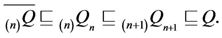An application of Part i of Theorem 4.1 then shows that 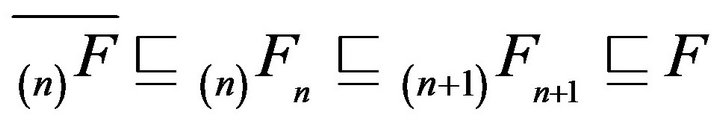for all Consquently,

(19)

where is the unique stationary distribution for The sequence is therefore tight and so

for all as The same is true for

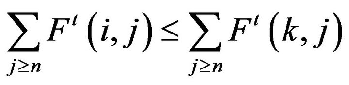
From (19), we observe that

for all

and so is at least as good an approximation to p as. Thus, any invariant measure derived from a north-west corner truncation of augmented in its last column is optimal for approximating.

As was pointed out in [7], the pointwise convergence of measures on a countable set can easily be extended to convergence in total variation. We therefore have the following result.

Theorem 4.2 Let be the -matrix of a positive recurrent, stochastically monotone Markov process on Let p be the stationary distribution of the minimal -function and denote the invariant distribution of an arbitrary north-west corner augmentation

by Furthermore, let be the

north-west corner truncation augmented in column n and take to be its invariant distribution. Then,

as The same is true of the sequence which is the optimal approximation in the sense that its tail mass more closely approximates that of.

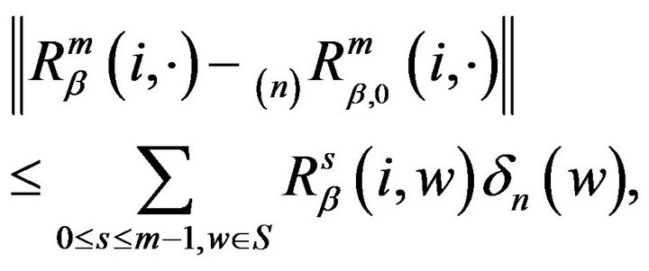
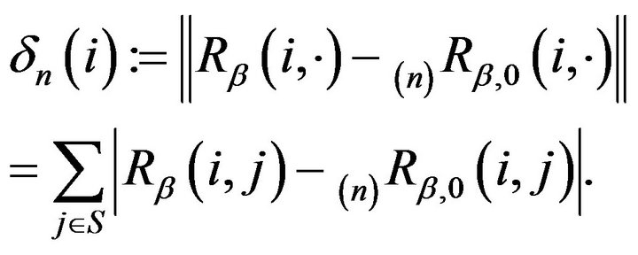
Proof: The fact that, for all and as was established in the preceding discussion. So too was the optimality of as an approximation to To prove convergence in total variation, fix an arbitrary finite Then, we obtain

The analogous statement holds for and the proof is completed by letting first and then tend to infinity.

As remarked in [6], will be strictly positive for sufficiently large n where a is an arbitrary state in Thus, contains a positive recurrent class to which n belongs. Computationally speaking, this means that any invariant distribution will suffice as an approximation to, provided n is sufficiently large.

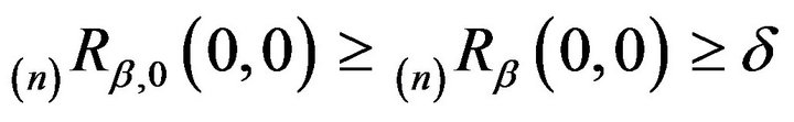
Finally, if n is large enough so that possesses a quasistationary distribution (n)r supported on a nondegenerate irreducible subset of then the sequence of distributions converges weakly to We can always find a sequence of irreducible sets such that 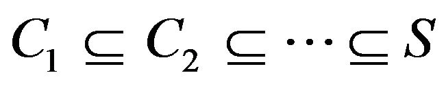and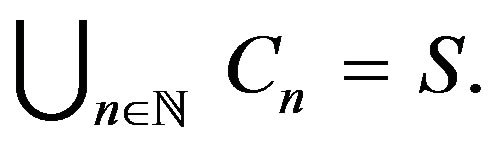

See Lemma 5.1 in [16] for a proof of this; the analogue for discrete-time Markov chains may be found in [3], Theorem 3.1.

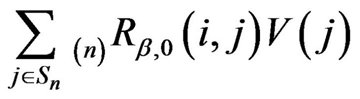
For a finite state Markov process, every quasistationary distribution is equivalent to a probabilitynormalised left eigenvector of its -matrix restricted to an ireducible class. In other words, If is a nonconservative -matrix on a finite state space S containing an ireducible class 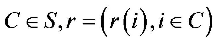is a quasistationary distribution on C for the process if and only if 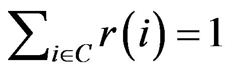and, for some

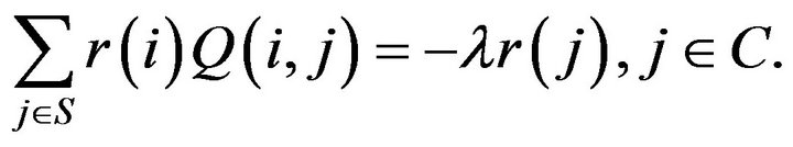
Note that by virtue of -theory, is strictly positive for all By convention, we extend r to by setting for If we then construct the linear augmentation as

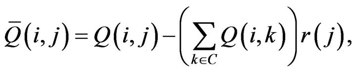(20)

it is not difficult to see that the invariant distribution for is unique and equivalent to

Now, let us return to the case of a countably infinite state space. Given n large, we may construct from

in the same manner as (20) using a left eigenvector 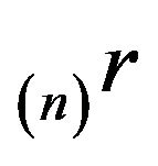of supported on an irreducible class The conditions of Theorem 4.2 are satisfied and so the sequence converges in total variation to the invariant distribution of This observation subsumes results concerning the truncation approximation of invariant distributions of birth-death processes and subcritical Markov branching processes, for example, see [16-18]. The convergence of quasistationary distributions of truncations to the invariant distribution of the original process also holds under the weaker conditions we discuss in the next two subsections.

4.2. Processes Dominated by Stochastically Monotone Processes

Now we shall consider a much larger class of Markov processes, namely those whose transition functions are stochastically dominated by a positive recurrent, stochastically monotone process. To begin, let be the stochastically monotone transition function of an irreducible, positive recurrent Markov process. Suppose that dominates a transition function F. We shall use and to denote the corresponding -matrices. As noted earlier, F must be positive recurrent and the invariant distributions and, corresponding to and respectively, satisfy.

Let and respectively denote the

north-west corner truncations of and augmented in the th column. By extending these in the analogous way to (18) and applying Part i of Theorem 4.1, we see that and are stochastically comparable.

Also, let be an arbitrary augmentation of an

north-west corner truncation ofand note that

whence 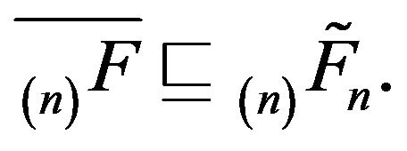From the previous subsection, 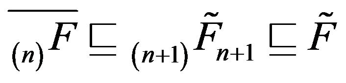for

Combining these, we obtain

which implies that

Thus, the sequence

is tight and componentwise as

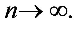
Convergence in total variation follows in the same way as in the proof of Theorem 4.2 and the same is true of

Thus we have proved the following result.

Theorem 4.3 Let be the -matrix of an irreducible Markov process which is dominated by a positive recurrent, stochastically monotone Markov process. Then,

as where p is the unique invariant distribution for and for constitutes an invariant distribution of an arbitrary north-west corner augmentation of

As the augmentation is a special case of

it follows from the theorem that as

However, unlike the situation in which F is stochastically monotone, it is not clear which of and provides the better approximation to

4.3. Finitely Perturbed Stochastically Monotone Markov Processes

Finally, we consider an even more general class of Markov processes which was introduced in [7]. We say that Q is a finite perturbation of if the two Q-matrices differ in at most a finite number of columns. Let be stochastically monotone and suppose without loss of generality that Q and differ in the first k columns. Let

and construct a

as follows:

Observe that is stochastically monotone. This is due firstly to the way in which the first k columns have been constructed from, and secondly to the agreement between the remaining columns of with the corresponding columns of the stochastically monotone. Now, satisfies (17) and so, by Theorem 4.1, the minimal -function F and-function are stochastically comparable. Direct application of Theorem 4.3 to and then yields the following result.

Theorem 4.4 Let be a finite perturbation of a Qmatrix whose minimal -function is irreducible, positive recurrent and stochastically monotone. Also, let p be the unique invariant distribution for and denote the invariant distributions of arbitrary north-west corner augmentations by. Then,

4.4. Example

Conrth-death process, whose tridiagonal

where 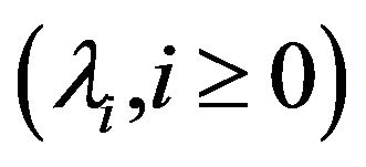are strictly positive birth rates and

are strictly positive death rates. Here, we take the state space S to be the set of non-negative integers. Such processes can be used to model queues having memoriless arrival and service times, simple circuitswitched teletraffic networks and buffers in computer networks, etc.

Let be the of an irreducible birth-death process. Then, it can be shown (see [1], Chapter 3) that

is regular if and only if

where and for. Now for

regular, the unique minimal transition function is positive recurrent if and only if and. The stationary distribution for is

where

Now, it is straight forward to verify that satisfies (17) and hence, by Theorem 4.1, is stochastically monotone. furthermore, by Theorem 4.2, we may use to approximate. Letting denote the north-west corner truncation on, augmentation in column n yields the matrix which differs from only in its element. More precisely,

andif either or. The stationary distribution corresponding to the augmentation is given by From this closed form expression, it can immediately be seen that

as since as

. Convergence in total variation then follows as in the proof of Theorem 4.2.

5. Conclusion

Here we have investigated procedures based on the augmentation of state-space truncations for approximating the stationary distributions of positive recurrent, continuous-time Markov processes on countably infinite state spaces. We have shown that approximation techniques first proposed for application to discrete-time markov chains are also efficacious in the continuous-time setting. Two classes of Markov process were considered: Exponentially ergodic processes and stochastically monotone processes. It was shown that the invariant distributions corresponding to the augmented

of finite statespace truncations of a

converge in total variation to the invariant distribution of the Markov process generated by that. It remains to study the speed of such convergence. An understanding of the convergence rate would enable the truncation size to be selected in order to guarantee that the measure approximates to a desired degree of accuracy.

6. Acknowledgements

This work was supported by the Center for Mathematical Modeling (CMM) Basal CONICYT Program PFB 03 and FONDECYT grant 1070344. AGH would like to thank Servet Martinez for interesting discussion on the truncation of stochastically monotone processes. AGH dedicates this article to co-author Richard Tweedie, who passed away after this work was started.

REFERENCES

- W. Anderson, “Continuous-Time Markov Chains: An Applications-Oriented Approach,” Springer Series in Statistics, Springer-Verlag, New York, 1991.
- E. Seneta, “Finite Approximations to Infinite Nonnegative Matrices I,” Proceedings of the Cambridge Philosophical Society, Vol. 63, No. 4, 1967, pp. 983-992. doi:10.1017/S0305004100042006
- E. Seneta, “Finite Approximations to Infinite Nonnega tive Matrices II: Refinements and Applications,” Proceedings of the Cambridge Philosophical Society, Vol. 64, No. 2, 1968, pp. 465-470. doi:10.1017/S0305004100043061
- E. Seneta, “Computing the Stationary Distribution for Infinite Markov Chains,” Linear Algebra and Its Applications, Vol. 34, 1980, pp. 259-267. doi:10.1016/0024-3795(80)90168-8
- D. Gibson and E. Seneta, “Monotone Infinite Stochastic Matrices and Their Augmented Truncations,” Stochastic Processes and Their Applications, Vol. 24, No. 2, 1987, pp. 287-292. doi:10.1016/0304-4149(87)90019-6
- D. Gibson and E. Seneta, “Augmented Truncations of Infinite Stochastic Matrices,” Journal of Applied Probability, Vol. 24, No. 3, 1987, pp. 600-608. doi:10.2307/3214092
- R. Tweedie, “Truncation Approximations of Invariant Measures for Markov Chains,” Journal of Applied Probability, Vol. 35, No. 3, 1998, pp. 517-536. doi:10.1239/jap/1032265201
- R. Tweedie, “Truncation Procedures for Nonnegative Matrices,” Journal of Applied Probability, Vol. 8, No. 2, 1971, pp. 311-320. doi:10.2307/3211901
- R. Tweedie, “The Calculation of Limit Probabilities for Denumerable Markov Processes from Infinitesimal Properties,” Journal of Applied Probability, Vol. 10, No. 1, 1973, pp. 84-99. doi:10.2307/3212497
- J. Kingman, “The Exponential Decay of Markov Transition Probabilities,” Proceedings of the London Mathematical Society, Vol. 13, No. 1, 1963, pp. 337-358. doi:10.1112/plms/s3-13.1.337
- D. Down, S. Meyn and R. Tweedie, “Exponential and Uniform Ergodicity of Markov Processes,” Annals of Probability, Vol. 23, No. 4, 1995, pp. 1671-1691. doi:10.1214/aop/1176987798
- R. Tweedie, “Criteria for Ergodicity, Exponential Ergodicity and Strong Ergodicity of Markov Processes,” Journal of Applied Probability, Vol. 18, No. 1, 1981, pp. 122-130. doi:10.2307/3213172
- S. Meyn and R. Tweedie, “Markov Chains and Stochastic Stability,” Springer-Verlag, London, 1993. doi:10.1007/978-1-4471-3267-7
- S. Meyn and R. Tweedie, “Computable Bounds for Convergence Rates of Markov Chains,” Annals of Applied Probability, Vol. 4, No. 4, 1994, pp. 981-1011. doi:10.1214/aoap/1177004900
- B. Kirstein, “Monotonicity and Comparability of TimeHomogeneous Markov Processes with Discrete State Space,” Statistics, Vol. 7, No. 1, 1976, pp. 151-168.
- A. Hart, “Quasistationary Distributions for ContinuousTime Markov Chains,” Ph.D. thesis, University of Queensland, Brisbane, 1997.
- L. Breyer and A. Hart, “Approximations of Quasistationary Distributions for Markov Chains,” Mathematical and Computer Modelling, Vol. 31, No. 10-12, 2000, pp. 69-79. doi:10.1016/S0895-7177(00)00073-X
- M. Kijima and E. Seneta, “Some Results for Quasistationary Distributions of Birth-Death Processes,” Journal of Applied Probability, Vol. 28, No. 3, 1991, pp. 503-511. doi:10.2307/3214486