Applied Mathematics
Vol. 3 No. 6 (2012) , Article ID: 20362 , 11 pages DOI:10.4236/am.2012.36100
Modeling and Analysis of a Single Species Population with Viral Infection in Polluted Environment
1IMS Engineering College, Adyatmik Nagar, Ghaziabad, India
2School of Mathematics and Allied Sciences, Jiwaji University, Gwalior, India
Email: sudipachauhan@gmail.com, misra_op58@yahoo.co.in
Received September 7, 2011; revised May 2, 2012; accepted May 9, 2012
Keywords: Virus Population; Single-Species Population; Hopf-Bifurcation; Stability
ABSTRACT
In this paper, a mathematical model is proposed to study the effect of pollutant and virus induced disease on single species animal population and its essential mathematical features are analyzed. It is observed that the susceptible population does not vanish when it is only under the effect of infection but in the polluted environment, it can go to extinction. Also, it has been observed that the replication threshold obtained, increases on account of pollutant concentration consequently decreasing the susceptible population. Further persistence results for the proposed model are obtained and the condition for the existence of the Hopf-bifurcation is derived. Finally, numerical simulation in support of analytical results is carried out.
1. Introduction
Pathogens such as viruses, bacteria, protozoan, and helminthes affect their host’s population dynamics [1-7]. It is now widely believed that disease and parasites are responsible for a number of extinctions on island and on large land masses. Theory on the effects of parasites on host population dynamics has received much attention and focused on issues such as how the parasite induced reduction of the host fecundity and survival rates change the host population dynamics, and how such dynamics be applied to predict threats to biodiversity in general and endangered species in particular [8,9]. Besides the study of effect of disease, effect of environmental pollution is also a great challenge in the study of the population dynamics in a polluted environment. A great quantity of the pollutant enters into the environment one after another which seriously threaten the survival of the exposed populations including human population. For a general class of single population models with pollutant stress, [10] obtained a survival threshold distinguishing between persistence in the mean and extinction of a single species under the hypothesis that the capacity of the environment is large relative to the population biomass, and that the exogenous input of pollutant into the environment is bounded. The threshold of survival for a system of two species in polluted environment was studied by [11]. Again, a spatial structure has been carried out by [12], to describe the dynamics of a population in a polluted environment and the sufficient criteria for the persistence and the extinction of the population are described. Many researchers have studied SIR model for different disease, such as dengue disease transmission [13]. Most recently, the bird flu, or H5N1, has garnered public attention for its potential not only to spread from chickens and other birds to humans, but also for the virus to mutate in a way that allows it to spread between humans. During the study period, bird flu killed just over half of the 145 people infected with the virus. In the absence of the virus the population is growing logistically according to the carrying capacity of the particular system but as the virus affects the species, its population starts decreasing and the population is divided into susceptible and infected population. It is well known fact that the virus multiply in the host body. This period when it multiply in the susceptible body is called the latent period and as the latent period gets over, it becomes infected and thus the disease spreads to the whole population resulting in the Deterioration of the population. But if along with this infection, if the population comes in contact with some toxicant directly with the food they intake like harmful chemicals then the situation gets worse [14]. Developed an extension of standard epidemiological models that describes the probability of disease spread among a given population of chicken. The model considered actual disease surveillance data gathered by health experts like the World Health Organization and looked for anomalies in the expected transmission rate versus the actual one. It is assumed that two viruses namely strain 1 and strain 2 causes the disease and long lasting immunity from infection caused by one virus may not be valid with respect to a secondary infection by the other virus. As a result ecologists acknowledge the importance of disease and parasite in the dynamics of the population [15-19]. Recently few interesting mathematical models with combined effects of disease and toxicant were studied [20- 22], for competing and prey predator dynamics. Keeping in view of the above, in this paper, we have proposed a mathematical model by considering the combined effect of both the infection and the toxicant through food intake and environmental toxicant. Many researchers have been done on the persistence of a biological system affected by infectious disease and the harmful toxicant separately, but here we have actually studied the combined effect of both disease and toxicant on a single population. This can be very useful for the researchers as it is not necessary that the system can have only one negative factor affecting it. This model is very helpful for plant population also which are infected by viruses and by environmental toxicant and the toxicant via food. Plant populations are affected by harmful toxicant like air pollutants which from combustion include sulphur dioxide and fluoride and those from photochemical reactions include complex nitrates and ozone and affect the plants. A few hundred plant viruses cause diseases known as tobacco, cucumber or tomato mosaics, potato leaf roll, raspberry ring spot, tulip flower breaking, barley yellow dwarf, etc. Several viroids cause diseases such as potato spindle tuber, cucumber pale fruit, hop and chrysanthemum stunt, etc.
2. Mathematical Model
The mathematical model that we are presenting in this paper is constrained to the following assumptions:
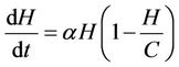
1) We have two populations viz. a single species animal population in terrestrial ecosystem denoted by symbol  at time t and a virus biomass, which are bacteriophages, denoted by symbol
  at time t.
2) In the absence of bacteriophages (i.e. viruses) the single species population density grows according to a logistic curve with carrying capacity  with an intrinsic birth rate constant
 :
:
 (1)
(1)
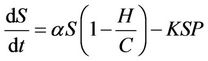
3) In the presence of virus biomass, we assume that total population  is composed of two population classes:
 , where
  is the susceptible population class, and
  is the infected population class.
4) It has been assumed that only susceptible population is capable of reproducing with logistic law. However, the infected population still contributes with susceptible population growth towards the carrying capacity.
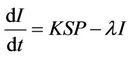
5) A susceptible population  becomes infected
  under the attack of many virus particles. Virus enters into susceptible individual, and then starts its replication inside the susceptible individual (now infected). Therefore, the evolution equation for the susceptible class
  according to the Equation (1) under assumptions 4) and 5) is:
 (2)
(2)
where,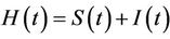 . In equation above
  represents effective animal population contact rate with viruses.
6) An infected individual  has a latent period, which is the period between the instant of infection and that of lysis, during which the virus reproduces inside the individual. The lysis death rate constant
  gives a measure of latency period T being
 . The lysis of the infected individual on the average, produces b virus particles
 , b is the virus replication factor.
7) The virus particles have a death rate constant , which accounts for all kinds of possible mortality of viruses due to enzymatic attack, pH dependence, temperature changes, UV radiation etc.
From the above assumptions, the model equations are:
 (3)
(3)
 (4)
(4)
 (5)
(5)
It has been observed that virus replication factor i.e. b plays an important role in shaping the dynamics of systems (3)-(5). If b is greater than some critical value then system exhibits the oscillatory behavior. Also, it has been established that systems (3)-(5) is uniformly persistent if  where
where . Further, to elaborate the effect of environmental pollution on single species population
  when it is already subjected to virus induced infection, we consider following assumptions:
8) We assume that pollutant enters into population via food which they intake and also from environment.
9) Pollutant losses from organism due to metabolic processing and other causes.
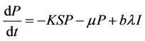
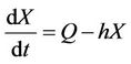
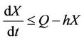
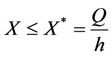
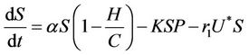
If Q is the constant exogenous input rate of the pollutant into environment then evolution equation for the concentration of environmental pollutant and for the organismal concentration of toxicant is given as:
 (6)
(6)
 (7)
(7)
where,  is the environmental concentration of the pollutant,
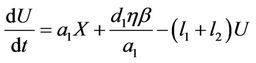
  is the organismal concentration of the pollutant. h is the loss rate of toxicant from environment, a1 is environmental pollutant uptake rate per unit mass organism, the uptake rate of pollutant in food per unit mass organism is denoted by second term in Equation (7);
 , is the concentration of the pollutant in resource,
  , is the average rate of the food intake per unit mass organism, d1, the uptake rate of pollutant in food per unit mass organism. l1 and l2 are organismal net ingestion and depuration rates of pollutant, respectively. The natural loss rate of pollutant from environment can be due to biological transformation, hydrolysis, volatilization, microbial degradation, including other processes. Thus the extended form of the systems (3)-(5) including Equations (6) and (7) is given as follows:
 (8)
(8)
 (9)
(9)
 (10)
(10)
 (11)
(11)
 (12)
(12)
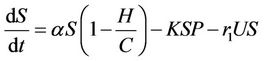
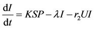
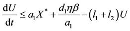
where, r1 and r2 are loss rates from susceptible and infected populations respectively due to effect of pollutant. In the next section, we will show that all the solutions of the Model (8)-(12) are bounded.
3. Boundedness and Equilibria
The boundedness of the solutions can be achieved by the following lemma.
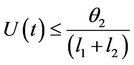
Lemma 3.1. All the solutions of the Model (8)-(12) will lie in the following region as 
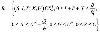
where
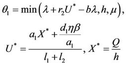
and C is the carrying capacity of the susceptible population.
Proof. Let us consider the function
then from Equations (9)-(11), we get
Let  then
then
then by usual comparison theorem [23], we get the following expression as 
 and hence
From (12), we get
Let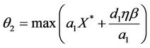 , then we get

then by usual comparison theorem [23], we get the following expression as 
From (11), we get
then by again usual comparison theorem, we get
This completes the proof of lemma.
Now, consider the following system:
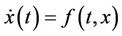 (13)
(13)
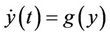 (14)
(14)
where, f and g are continuous and locally Lipschitz in x in , and solutions exists for all positive time. Equation (14) is called asymptotically autonomous with limit equation (13) if
  as
as  uniformly for all x in
 .
.
Lemma 3.2. Let e be a locally asymptotically stable equilibrium of (14) and ω be the ω-limit set of a forward bounded solution  of (13). If ω contains a point y0 such that the solutions of (14), with
  converges to e as
 , then
  i.e.
i.e.  as
as .
.
Corollary. If the solutions of the system (13) are bounded and the equilibrium e of the limit system (14) is globally asymptotically stable than any solution  of the system (19) satisfies
  as
as .
.
The Equations (11) and (12) can be solved explicitly and we obtain
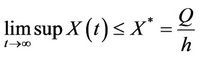
and
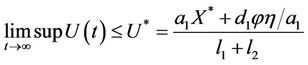
Thus, on applying above corollary in systems (8)-(12) we get the following equivalent asymptotic autonomous system:
 (15)
(15)
 (16)
(16)
 (17)
(17)
To predict the dynamical behavior of the systems (8)- (12) it is sufficient to study the behavior of the systems (15)-(17), since the behavior of the systems (15)-(17) near to the steady states is similar to the behavior of the systems (8)-(12). Now, we rescale the systems (15)-(17) using following non-dimensionalised quantities: ,
,  ,
,  and
and , we get
 (18)
(18)
 (19)
(19)
 (20)
(20)
where,
 ,
,  ,
,  ,
,  ,
, 
and ,
,  ,
,  ,
,  ,
, . All the initial conditions for (18)-(20) may be any point in the non-negative orthant of
  of
of  and
and  is defined as the interior of
 . We will use notation t instead of notation
  for the convenience in rest of the paper. Systems (18)-(20) has three feasible equilibrium points, trivial equilibrium point
 , disease free equilibrium point
  and a interior equilibrium point
 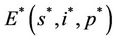 where
where
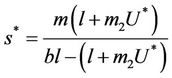
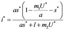
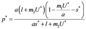
and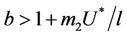 ,
, . Whenever
 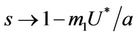 then
then  and
and , i.e. in this case positive equilibrium point
  approaches to disease free equilibrium state E1 in polluted environment. Now, we move to the biological relevant parameter b i.e. the virus replication factor. This parameter plays an important role in shaping the dynamics of the system. We see that as
 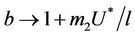 then
then , and in pollution free environment, we have
  as
as . It is readily clear that lower limit for virus replication factor has been increased to
  from
from  due to presence of the toxicant into the environment. Of course, the range of virus replication factor has become shorter
  in polluted environment as compared to
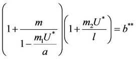
  in pollution free environment for the existence of the interior equilibrium point. It is clear that for increasing value of U* the lower limit of parameter b for the existence of positive equilibria of system increases, and we know as b increases then
  is monotonically decreasing but constrained to the range
  and it reaches the value
 at
at
 (21)
(21)
and in absence of toxicant we have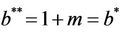 . Nowit is clear that
 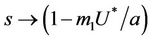 as
as  in polluted environment and
  as
as . Thus, positive equilibria
  is not feasible when ever
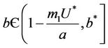 .
.
In this case, we have stable boundary equilibrium point E1 at which epidemic cannot occur and the trivial equilibrium E0 state remains unstable saddle point for any parameter value provided . Increasing b further i.e.
 ; we see that
 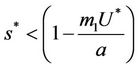 and
and
 ,
, . Hence, when the virus replication factor is larger than
 , then interior equilibria will exists. We can summarize the above result in following proposition.
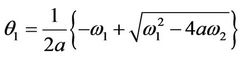
Proposition 1. Whenever, 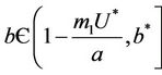 then equilibria of the system (18)-(20) are E0 and E1, and whenever
  then the positive equilibria
  is feasible. Moreover, as
  then
then  and at
  we have
 . It is clear by the above discussion that for the existence of positive equilibria the virus replication factor i.e. b should be much higher i.e.
  in the polluted environment instead of pollution free environment where
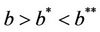 . Also, as
  increases then
  increases and simultaneously
  decreases. Thus, amount of toxicant in environment plays an important role in co-existence of all species in the systems (18)-(20).
4. Local Stability and Bifurcation Analysis
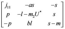
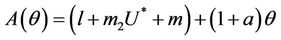
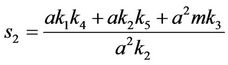
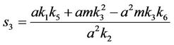
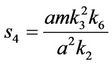
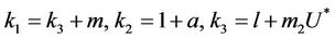
In this section we will discuss local stability analysis of the systems (18)-(20). Moreover, condition for the existence of Hopf-bifurcation has also been discussed in this section. The jacobian matrix for the systems (18)-(20) is given as:
where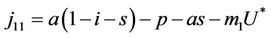 . At trivial equilibrium point
  we have:
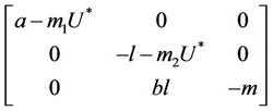
We have following eigen values corresponding to :
:
and . It is clear that jacobian of the system (18)- (20) corresponding to vanishing equilibria
  is attracting in s direction when
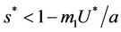
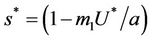
 , which means that the susceptible population can vanish only when it’s intrinsic growth rate become smaller than the death due to pollutant. On the other hand if
  then susceptible population can never vanish. It has been already studied that in pollutant Free State, jacobian of the systems (18)-(20) corresponding to
  is always repulsive in s direction. Thus, it is clear that due to effect of toxicant, the susceptible population can vanish. While, on the other hand in pollutant free environment susceptible population in systems (15)-(17) can never vanish. According to eigen values it has been observed that Jacobian J corresponding to trivial equilibria
  is repulsive in s direction when
 , and attracting in i and p direction. Thus, the above discussion shows that
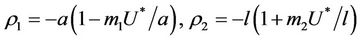
  is an unstable saddle point. We know discuss the disease free equilibrium point E1, when
 , then corresponding to this equilibrium point we have the following jacobian matrix:
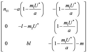
where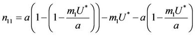 .
.
Then, we have following eigen values of :
:  and
and  and
and  are roots of the following quadratic:
where

It is clear that , and
, and  can be rewritten in the following form:

where  is first point in positive equilibrium point
 : Now, if
  and
and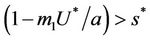 , then E1 is a saddle point, and when
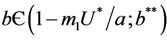 , then we have
  and therefore positive equilibrium point
  is not feasible. Thus, for the situation
 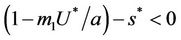 equation
  has two real and negative roots. Now, when
  then
then
 and the disease free equilibrium point E1 has one vanishing eigen value and two real and negative eigen values:
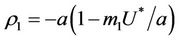 ,
,  and
and , i.e. in this case E1 is critically asymptotically stable. Finally, when
  and
and 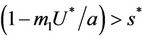 then positive equilibria E* exists and E1 become repulsive.
The above results can be summarized as in the form of the following lemma.
Lemma 4.1. For the systems (18)-(20), the trivial equilibrium point E0 is always an unstable saddle point if . The disease free equilibria E1 in polluted environment is locally asymptotically stable point if
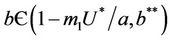 ; i.e. when E* is not feasible. At
 , E1 become critically stable. Whereas, when E* is feasible i.e. for
 , E1 is repulsive.
Now, we will discuss the local behavior of the flow of the system (18)-(20) near to the positive equilibrium point E*. Let us consider  and
and . The jacobian of the system (18)-(20) corresponding to positive equilibrium point
  is given as:
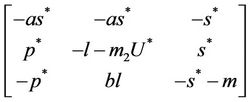
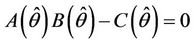
then the characteristic equation corresponding to above jacobian  is given as:
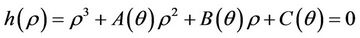
where
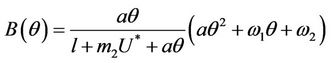
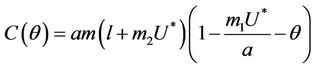
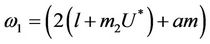
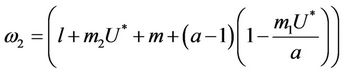
Here,  and
and  for all
 , and for
  we have following two cases:
1) , in this case
  for all
2)  in this case
  for all
 , and
, and  for all
 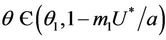 and
and  at
at  where
where
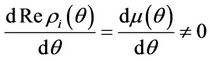
which is the root of . The Hurwitz criterion gives a necessary and sufficient condition for local asymptotic stability of E*.
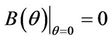
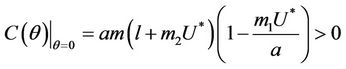
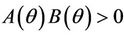
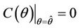
Routh-Hurwitz criterion and Hopf-bifurcation: For any , E* is locally asymptotically stable if and only if:
 ,
, 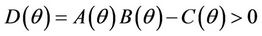 and
and .
.
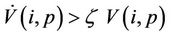
In the following we give for our case the definition of a simple Hopf bifurcation. Assume that the positive equilibrium depends E* of the system (18)-(20) smoothly depends on the parameter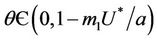 . If there exists
 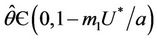 such that 1) A simple pair of complex conjugate eigen values of Equation (22) exists, say
  and
and
 , such that they become purely imaginary at
 , i.e.
  and
and whereas the other eigenvalue
  at
at  remains real and negative. And2) At
 , i = 1, 2, we must have
Then at  we have a simple Hopf-bifurcation. Without knowing eigenvalues, [15] proved that if
 ,
,  and
and  are smooth functions of
  in an open interval of
  such that
 ,
,  ,
, 
and at 
then simple Hopf-bifurcation occurs at . According to the above results we can prove the Theorem 4.1.
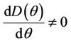
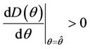
Theorem 4.1. Assume that  for all
 , then a single Hopf-bifurcation occurs at the unique value
  for decreasing
 , i.e. the positive equilibria E* is asymptotically stable in
  and unstable in
 .
.
Proof. Coefficients of the characteristic Equation (22) for positive equilibria E* are ,
,  and
and , and when
  then all these coefficients are positive. Now, we look at
 . Since
 and
and
then we have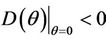 . Further at
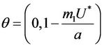 ,
,  ,
,  and hence
 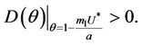 Since
Since  is continuous on
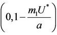 , then a value
 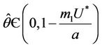 must exists at which
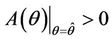 ,
,  ,
, . The value at
 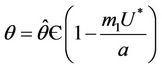 is unique because
  is monotone increasing and
  is monotone decreasing in
  Further, it is easy to check that at
 ,
,
Hence  in
in , and according to Routh-Hurwitz criterion E* is asymptotically stable
 . Furthermore, at
 , we have a simple Hopf-bifurcation towards periodic solutions for decreasing θ, being
  in
in , i.e. E* is unstable when
 . This finishes the proof.
Suppose,  , i.e. there exists
 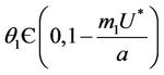 such which
and  for
for  and
and  for
for  . Now, in this case we can prove the Theorem 4.2.
Theorem 4.2. Assume that  , i.e. there exists
  at which
  Then, there exists a unique value
  at which a simple Hopf bifurcation occurs for decreasing
 . Therefore, the positive equilibria E* is asymptotically stable in
  and unstable in
 .
.
Proof. Let us remark that  in
in  and
and  in
in  with
with . Then,
  in
in  Furthermore,
  at
at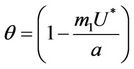 . Since,
  is continuous on
  , then there exists a
  such that
 . The uniqueness of
  follows from the remark that
  is monotone increasing and
  is monotone decreasing functions of
  in
in . Hence,
  in
in , and
, and  in
in  with
with  i.e. at
  we have simple Hopf-bifurcation, with E* asymptotically stable in
 , and unstable in
 . This finishes the proof.
5. Global Stability and Persistence
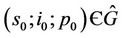
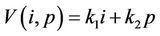
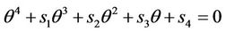
In this section, we will establish global stability and persistence results for the system (18)-(20). We claim that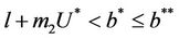 , where
the boundary equilibria E1 is globally asymptotically stable with respect to .
.
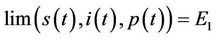
Theorem 5.1. If 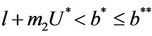 then the boundary equilibrium point E1 is globally asymptotically stable in
 .
.
Proof. Let G be the set of . We proved that any solution of systems (18)-(20) starting outside G either enters into G at some finite time, say
  and then it remains in its interior G for all
  or tends to the boundary equilibrium E1. It is therefore sufficient to prove that E1 is asymptotically stable with respect to G to prove global asymptotic stability in
 . Let
. Let
 , consider a scalar function
 , such that
where k1 and k2 are real positive numbers. Then from Equations (18)-(20) we arrive at:
 (25)
(25)
In Equation (25) we can choose , then we get:
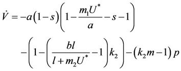
Furthermore, if we choose k2 in such a way that
then from Equation (26) we get:
 (27)
(27)
The above Inequality (27) holds for any ,
,  and
and  in
in . However, in this case we have:

It is straightforward to show that the largest invariant set in M is E1, by the well known Lasalle-Lyapunov theorem, we again show that E1 is globally asymptotically stable when . This finishes the proof.
Assume now that positive equilibria E* is feasible i.e. , thus we can prove the following theorem about E1.
Theorem 5.2. If  then there are no
 (where
  is interior of
 ) such that
 as
as .
.
Proof. Let us consider following function:
where , (i = 1, 2) which is of course positive in G since
  and
and . let
. let  be a ε-neighborhood of E1 in G. Then from Equationa (19) and (20) we get:
 (28)
(28)
or
 (29)
(29)
where the inequality on the right of the Equation (29) holds true in  Positive definiteness of
  in
in  requires that
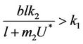
and
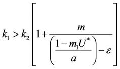
and this in turns requires that
 (30)
(30)
when,  then, for all
 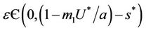 Inequality (30) holds true, thus for the choice of k1 and k2 Inequality (29) holds true. Hence, there is
  such that for the above choice of k1 and k2, we get:
in Iε. This finishes the proof.
Moreover, it has been observed in the light of above theorem that, when  then boundary equilibria E1 is uniformly strong repeller, and in this case positive equilibria E* is uniformly persistent.
6. Numerical Example
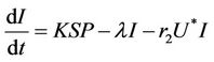
Let us we consider following set of parameters a = 10, l = 24.628, m = 14.925, m1 = 0.01, m2 = 0.011, Q = 1, h = 0.1, a1 = 1, d1 = 0:21, θ = 1, β = 0:12, (l1 + l2) = 0:5.
Then we get X* = 10 and U* = 20.05. In this case, interior equilibrium point of the system (18)-(20) is E* = (0.3862, 0.0799, 5.1388). Since, we have considered  as a Hopf-bifurcation parameter, thus at
  we have:
where  is the positive and real root of the following equation:
 (31)
(31)
where
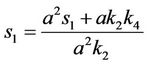
and,
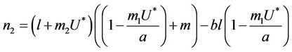
Thus, for the above numerical data we have following positive root of the equation  = 0.1568 and corresponding to this value of θ, we have threshold replication factor b = 97.0463 and b** = 16.3759. So, we have the following numerical observations:
1) if b Є (k6, 16.3759) then steady state E1 is globally asymptotically stable, and interior equilibrium point E* of the systems (18)-(20) does not exist (Figure 1).
2) if b Є (16.3795, 1), then interior equilibrium point E* of the systems (18)-(20) exists.
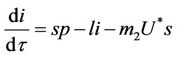
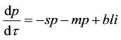
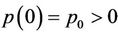
Moreover, if b Є (16.3759, 97.0463), then equilibria E* is locally asymptotically stable (Figures 2 and 3). Whenever b ≥ 97.0463, then E* is locally asymptotically unstable, and in this case systems (18)-(20) exhibits small amplitude Hopf-type oscillations around steady state E* (Figures 4 and 5). Now, we increase exogenous input rate of the pollutant in the systems (18)-(20), suppose increased exogenous input rate of the pollutant is Q = 5. Then we have:
X* = 50, U* = 100.0504 and E* = (0.4003, 0.0673, 4.3244), b** = 18.3701,  = 0:1452,
  = 100.4832.
In this case, we have following observations:
1) if b Є (k6, 18.3701), then E1 is globally asymptotically stable and, E* is not feasible in this situation.
2) if b Є (18.3701, ) then steady state E* is feasible, and moreover, E* is locally asymptotically stable when b Є (18.3701, 100.4832), further, as b ≥ 100.4832, then system exhibits small amplitude oscillations around E*.
From both the above numerical observations, it is clear that due to effect of toxicant bifurcation threshold  comes down as environmental pollutant increases. On the other hand, b** increases as environmental pollutant increases, which in turn, conclude that as environmental pollutant increases then system would have co-existence of all constituent units i.e. existence of interior equilibrium point for higher values of virus replication factor b
Figure 1. E1 is globally asymptotically stable.
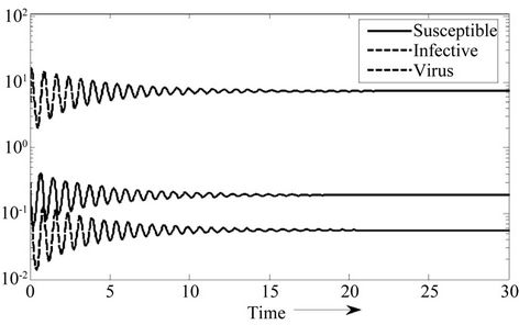
Figure 2. E* is locally asymptotically stable.
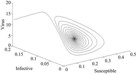
Figure 3. E* is locally asymptotically stable (Phase plane).
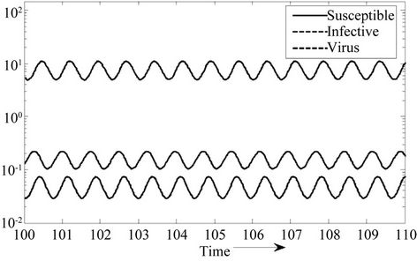
Figure 4. E* is locally unstable.
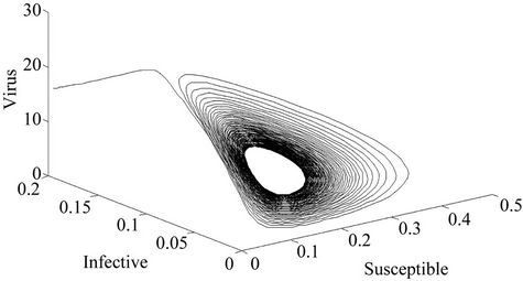
Figure 5. E* is locally unstable (Phase plane).
as compared to the case when pollutant is not present in the system.
7. Conclusion
A mathematical model for single species population which is infected by virus induced disease in a polluted environment is studied. We have studied the local and global behavior of the flow of the system around possible steady states. It has been established that boundary equilibria i.e. E1 is the globally asymptotically stable. Further, as boundary equilibria E1 become strongly repeller then flow of the system is persistent towards the positive equilibria E*. E0 is attractor when a < m1U* i.e. the intrinsic growth rate of susceptible population is less than the death due to pollutant otherwise it is unstable saddle point. It has been found that virus replication factor plays an important role in shaping the dynamics of the system in both the polluted and fresh environment. Further, when the effect of pollution is not considered then it has been established that susceptible population can never vanish, while, on the other hand when the effect of the environmental pollution has been considered then susceptible population can vanish if amount of the environmental pollutant is higher than a certain level. Furthermore, we have traced out two basic effects of environmental pollutant on single species when it is already subjected to some virus induced disease. One of them is that due to effect of pollutant equilibrium level of population goes down as organismal toxicant increases, which is a generally known effect. The second effect is that due to presence of pollutant, threshold of virus replication factor increases which in turn again depress the susceptible population density level. Moreover, it has been established that system exhibits oscillatory behavior as virus replication factor increases by a certain threshold level. We have established the existence of the oscillatory behavior of the solutions of the system using Hopf-bifurcation technique. Global behavior of the system has also been discussed using Lyapunov-LaSalle principle and persistent technique. Finally, a numerical example has also been added in support to analytical results.
REFERENCES
- R. M. Anderson and R. M May, “Regulation and Stability of Host-Parasite Population Interactions I: Regultory Processes,” Journal of Animal Ecology, Vol. 47, 1978, pp. 219-247. doi:10.2307/3933
- R. M. Anderson and R. M. May, “The Invasion, Persistence, and Spread of Infectious Disease within Animal and Plant Communities,” Transactions of the Royal Society of London, Vol. B 314, No. 1167, 1986, pp. 533-570.
- R. M. May and R. M. Anderson, “Regulations and Stability of Host-Parasite Population Interactions II, Destabilizing Processes,” Journal of Animal Ecology, Vol. 47, 1978, pp. 249-267. doi:10.2307/3934
- H. W. Hethcote and S. A. Levin, “Periodicity in Epidemiological Models,” In: L. Gross, T. G. Hallam and S. A. Levin, Eds., Applied Mathematical Ecology, SpringerVerlag, Berlin, 1989, pp. 193-211. doi:10.1007/978-3-642-61317-3_8
- M. Begon and R. G. Bowers, “Beyond Host-Parasite Dynamics,” In: B. T. Grenfell and A. P. Dobson, Eds., Ecology of Disease in Natural Populations, Cambridge University Press, Cambridge, 1995, pp. 479-509.
- B. T. Grenfell and A. P. Dobson, Eds., “Ecology of Disease in Natural Populations,” Cambridge University press, Cambridge, 1995.
- H. W. Hethcote, W. Wang and L. Yi, “Species Coexistence and Periodicity in Host-Host Pathogen Model,” Journal of Mathematical Biology, Vol. 51, No. 6, 2005, pp. 629-660.
- T.-W. Hwang and Y. Kuang, “Deterministic Extinction Effect of Parasite on Host Populations,” Journal of Mathematical Biology, Vol. 46, 2003, pp. 17-30. doi:10.1007/s00285-002-0165-7
- H. Mccallum and A. P. Dobson, “Detecting Diseases and Parasite Threats to Endangered Species Ecosystems,” Trends in Ecology and Evolution, Vol. 19, 1995, pp. 190-194. doi:10.1016/S0169-5347(00)89050-3
- M. Zhien, B. J. Song and T. G. Hallam, “The Threshold of Survival for the System in Fluctuating Environment,” Bulletin of Mathematical Biology, Vol. 57, No. 3, 1989, pp. 311-323.
- H. P. Liu and M. Zhien, “The Threshold of Survival for the System of Two Species in a Polluted Environment,” Journal of Mathematical Biology, Vol. 30, No. 1, 1991, pp. 49-61.
- L. Zhan, Z. S. Shun and W. Ke, “Persistence and Extinction of Single Population in a Polluted Environment, Electronic,” Journal of Differential Equations, Vol. 108, 2004, pp. 1-5.
- N. Nuraini, E. Soewono and K. A. Sidarto, “A Mathematical Model of Dengue Internal Transmission Process,” Journal of Indonesia Mathematical Society, Vol. 13, No. 1, 2007, pp. 123-132.
- N. M. May, “Los Alamos Mathematical Model Gauges Epidemic Potential of Emerging Diseases,” LOS ALAMOS, New Mexico, 27 May 2008.
- W. M. Liu, “Criterion of Hopf-Bifurcation without Using Eigenvalues,” Journal of Mathematical Analysis and Application, Vol. 250, 1994.
- D. Greenhalgh and M. Haque, “A Predator-Prey Model with Disease in Prey Species Only,” Mathematical Methods of Applied Sciences, Vol. 30, 2007, pp. 911-929. doi:10.1002/mma.815
- K. P. Hadeler and H. I. Freedman, “Predator-Prey Populations with Parasitic Infection,” Journal of Mathematical Biology, Vol. 27, No. 6, 1989, pp. 609-631.
- M. Haque and E. Venturino, “The Role of Transmissible Disease in Holling-Tanner Predator-Prey Model,” Theoritical Population Biology, Vol. 70, No. 3, 2006, pp. 273-863.
- E. Beltrami and T. O. Carroll, “Modelling the Role of Viral Disease in Recurrent Phytoplankton Blooms,” Journal of Mathematical Biology, Vol. 32, 1994, pp. 857- 863. doi:10.1007/BF00168802
- S. Sinha, O. P. Misra and J. Dhar, “Study of a Prey- Predator Dynamics under the Simultaneous Effect of Toxicant and Disease,” The Journal of Nonlinear Analysis and its Applications, Vol. 1, No. 2, 2008, pp. 102-117.
- S. Sinha, O. P. Misra and J. Dhar, “A Two Species Competition Model under the Simultaneous Effect of Toxicant and Disease,” Non-Linear Analysis-Real World Application, Elsevier Publication, Vol. 11, 2010, pp. 1131-1142.
- S. Sinha, O. P. Misra and J. Dhar, “Modeling a Predator Prey System with Infected Prey in Polluted Environment,” Applied Mathematical Modeling, Elsevier Publication, Vol. 34, 2010, pp. 1861-1872.
- J. K. Hale, “Ordinary Differential Equations,” 2nd Edition, Kriegor, Basel, 1980.