Intelligent Control and Automation, 2010, 1, 48-58
doi:10.4236/ica.201.11006 Published Online August 2010 (http://www.SciRP.org/journal/ica)
Maximizing of Asymptomatic Stage of Fast Progressive
HIV Infected Patient Using Embedding Method
Hassan Zarei, Ali Vahidian Kamyad, Sohrab Effati
Department of Applied Mathematics, Ferdowsi University of Mashhad, Mashhad, Iran
Received July 7, 2010; revised July 15, 2010; accepted July 23, 2010
Abstract
A system of ordinary differential equations, which describe various aspects of the interaction of HIV with
healthy cells in fast progressive patient, is utilized, and an optimal control problem is constructed to prolong
survival and delay the progression to AIDS as far as possible, subject to drug costs. Optimal control problem
is approximated by linear programming model using measure theoretical approach and suboptimal combina-
tions of reverse transcriptase inhibitor (RTI) and protease inhibitor (PI) drug efficacies are proposed. The
Comparison of healthy CD4+ T-cells counts, virus particles and immune response, before and after the
treatment is introduced.
Keywords: HIV Model, Optimal Control, Measure Theory, Linear Programming
1. Introduction
Human Immunodeficiency Virus infects CD4+ T-cells,
which are an important part of the human immune sys-
tem, and other target cells. The infected cells produce a
large number of viruses. Medical treatments for HIV
have greatly improved during the last two decades.
Highly active antiretroviral therapy (HAART) allows for
the effective suppression of HIV-infected individuals and
prolongs the time before the onset of Acquired Immune
Deficiency Syndrome (AIDS) for years or even decades
and increase life expectancy and quality to the patient but
antiretroviral therapy cannot eradicate HIV from infected
patients because of long-lived infected cells and sites
within the body where drugs may not achieve effective
levels [1-3]. HAART contain two major types of
anti-HIV drugs, reverse transcriptase inhibitors (RTI)
and protease inhibitors (PI). Reverse transcriptase in-
hibitors prevent HIV from infecting cells by blocking the
integration of the HIV viral code into the host cell ge-
nome. Protease inhibitors prevent infected cells from
replication of infectious virus particles, and can reduce
and maintain viral load below the limit of detection in
many patients. Moreover, treatment with either type of
drug can also increase the CD4+ T-cell count that are
target cells for HIV.
Many of the host–pathogen interaction mechanisms
during HIV infection and progression to AIDS are still
unknown. Mathematical modeling of HIV infection is of
interest to the medical community as no adequate animal
models exist in which to test efficacy of drug regimes.
These models can test different assumptions and provide
new insights into questions that is difficult to answer by
clinical or experimental studies. A number of mathe-
matical models have been formulated to describe various
aspects of the interaction of HIV with healthy cells, See
[4]. The basic model of HIV infection is presented by
Perelson et al. [5] that contain three state variables
healthy CD4+ T-cells, infected CD4+ T-cells and con-
centration of free virus. Another model is presented in [6]
that although maintaining a simple structure, the model
offers important theoretical insights into immune control
of the virus based on treatment strategies Furthermore
this modified model is developed to describe the natural
evolution of HIV infection, as qualitatively described in
several clinical studies [7].
Some authors use mathematical model for HIV infec-
tion in conjunction with control theory to achieve appro-
priate goals, by incorporating the effects of therapy on an
HIV-infected individuals. For example, these goals my
be maximizing the level of healthy CD4+ T-cells and
minimizing the cost of treatment [8-12], maximizing
immune response and minimizing both the cost of treat-
ment and viral load [13,14], maximizing both the level of
healthy CD4+ T-cells and immune response and mini-
mizing the cost of treatment [15], Maximizing the level
of healthy CD4+ T-cells while minimizing both the side
effects and drug resistance [16] and maximizing survival

H. ZAREI ET AL.
49
time of patient subject to drug cost [17] and etc.
The papers [18-21] consider only RTI medication
while the papers [22,23] consider only PIs. In [24-27] all
effects of a HAART medication are combined to one
control variable in the model. In [13,28-31] dynamical
multidrug therapies based on RTIs and PIs are designed.
In this paper, we consider a mathematical model of
HIV dynamics that includes the effect of antiretroviral
therapy, and perform an analysis of optimal control re-
garding appropriate goal.
The paper is organized as follows. In Section 2, the
underlying HIV mathematical model is described. Our
formulation of the control problem which attempts to
delay appearance of AIDS as far as possible is described
in Section 3. Formulated optimal control problem is ap-
proximated by linear programming (LP) problem. Re-
lated procedure is described in Section 4. Numerical re-
sults obtained from using LP model are presented in Sec-
tion 5. Finally Section 6 is assigned to concluding re-
marks.
2. Presentation of a Working Model
In this paper, the pathogenesis of HIV is modeled with a
system of ordinary differential equations (ODEs) de-
scribed in [7]. This model can be viewed as an extension
of basic HIV Models of Perelson et al. [5].
x
dx rxv

 
 (1)
y
rxv ayyz


 (2)
wcxywqyw bw
 (3)
zqywhz
 (4)

1P vkuy v

 
 (5)
0
R
rru
 (6)
Most of the terms in the model have straightforward
interpretations as following:
The first equation represents the dynamics of the con-
centration of healthy CD4+ T-cells (x). The healthy
CD4+ T-cells are produced from a source, such as the
thymus, at a constant rate λ, and die at a rate dx. The
cells are infected by the virus at a rate rxv. The second
equation describes the dynamics of the concentration of
infected CD4+ T-cells (y). The infected CD4+ T-cells
result from the infection of healthy CD4+ T-cells and die
at a rate ay and killed by cytotoxic T-lymphocyte effec-
tors CTLe(z) at a rate ρyz. The population of CTLs is
subdivided into precursors or CTLp (w), and effectors or
CTLe (z). Equations (3)-(4) describe the dynamics of
these compartments. In accordance with experimental
findings [32] establishment of a lasting CTL response
depends on CD4+ T-cell help, and that HIV impairs T
helper cell function. Thus, proliferation of the CTLp
population is given by cxyw and is proportional to both
virus load (y) and the number of uninfected T helper
cells (x). CTLp differentiation into effectors occurs at a
rate cqyw. Finally, CTLe die at a rate hz. Equation (5)
describes the dynamics of the free-virus particles (v).
These free-virus particles are produced from infected
CD4+ T-cells at a rate ky and are cleared at a rate τv.
Model also contain an index of the intrinsic virulence or
aggressiveness of the virus (r). This index increases line-
arly in the case of an untreated HIV-infected individual,
with a growth rate that depends on the constant r0 Finally
Equation (6) describes the dynamic of this index. In
model variables uP and uR denotes protease inhibitors (PI)
and reverse transcriptase inhibitors (RTI), respectively.
uR reduces infection rate of healthy CD4+ T-cells by
reducing the growth rate of the aggressiveness of the
virus (r) and uP prevents virus production by reducing
the production rate from infected CD4+ T-cells.
The model has several parameters that must be as-
signed for numerical simulations. The descriptions, nu-
merical values and units of the parameters are summa-
rized in Table 1. These descriptions and values were
taken from [7]. We note that Equations (1)-(6) with these
parameters, model dynamics of fast progressive patients
(FPP).
3. Optimal Control Formulation
In clinical practice, Anti-retroviral therapy is initiated at
t0, the time at which CD4+ T-cell counts reach 350
cells/μl. The transition from HIV to AIDS occurred when
patients CD4+ T-cell count falls below 4AIDS CD

around 200 cells/μl. Our aim is to propose drug regimen
Table 1. Parameter Values for the HIV model.
ParametersValue/Unit Description
λ 7 cellsµl-1day-1 Healthy CD4+ Production
d 7 × 10-3 day-1 Healthy CD4+ clearance
a 0.0999 day-1 Infected CD4+ clearance
ρ 2 µlcells-1 day-1 Infected CD4+ kill
c 5 × 10-6 µl2cells-2day-1 CTLp proliferation
q 6 × 10-4 µlcells-1day-1 CTLp differentiation
b 0.017 day-1 CTLp clearance
h 0.06 day-1 CTLe clearance
k 300 copiesml-1cells-1 µlday-1 Virus production
τ 0.2 day-1 Virus clearance
r0 10-9 copies-1ml day-2 Virulence growth

H. ZAREI ET AL.
50
to maximize asymptomatic stage time or equivalently
prolong survival and delays the progression to AIDS as
far as possible, subject to drug costs. This can be mod-
eled as follows:
Assume that the onset of AIDS occurs after time
f
t.
Hence we should have:


0
4,4,,
f
AIDSAIDS f
x
tCD xtCDttt




(7)
We follow [8] and [22] in assuming systemic costs of
the PI and RTI drugs treatment is proportional to 2()
P
ut
and 2()
R
ut at time t respectively. Therefore Overall cost
of the PI and RTI drugs treatment is
0
2()
f
P
t
tutdt
 and
0
2()
f
R
t
tutdt
 respectively and overall cost of treatment is
given by
00
22
() ()
ff
PR
tt
tt
utdt utdt  

. Because symmetric
costs for two types of drugs are in different scale, coeffi-
cient σ is set to balance them. Administration of drugs in
high dose, are toxic to the human body. Moreover emer-
gence of drug resistant strains is one of the basic com-
plications in drug treatments. Many authors have ignored
drug resistance issues, since fixing a maximum cost for a
drug regime is equivalent to only administering a limited
amount of chemotherapeutic agent. If that limited
amount is chosen to be sufficiently small positive

, the
risk of drug resistance can be largely ignored. Therefore
we impose following constraint on drug cost:
 

0
22
f
PR
t
tut utdt

 
 (8)
Setting, (, ,,,,)
x
ywzvr

 and ()(,)
P
R
utu u the
differential Equations (1)–(6) can be represented in a
generalized form as:
 


1156
156 224
12323 3
23 4
25
0
,,
1P
R
d
a
cqb
tgttut qh
ku
ru


 

 
  



















(9)
Now with respect to above descriptions and (7) and (8)
the optimal drug regime problem can be stated as fol-
lows:
0
,
max f
f
t
t
ut dt
 (10)
subject to

,,
g
tu 
 (11)
 


0
22
f
PR
t
tut utdt




 (12)




100 1
,4
f
AIDS
ttCD 

 (13)


10
4, ,
AIDS f
tCD ttt 



(14)
We refer to this time optimal control problem as
TOCP. Some problems may arise in the quest for the
optimal solution. For example, may not exist control
function (. )u and corresponding state (.)

and final
time
f
t that satisfy in (11)-(14). In order to overcome
these difficulties in the next section we transfer the
TOCP into a modified problem in measure space.
4. Approximation of TOCP by Linear
Programming Model
Using the measure theory for solving optimal control
problems based on the idea of Young [33], which was
applied for the first time by Wilson and Rubio [34], has
been theoretically established by Rubio in [35]. Then the
method has been extended and improved by Mehne et al.
[36] for solving time optimal control problems that leads
to approximation of problem by linear programming (LP)
model. We shall follow their approach here.
4.1. Transformation to Functional Space
We assume that state variable (.)

and control input
(.)u, get their values in the compact sets 1 AA


6
6
A and 2
12
UUU

, respectively. Set
0,
f
J
tt




.
Definition 4.1.1. We define a triple ,,
f
pt u 

 to
be admissible if the following conditions hold:
1) The vector function (.)

be absolutely continuous
and belongs to
A
for all tJ.
2) The function (.)u takes its value in the set U
and is Lebesgue measurable on
J
.
3) p satisfies in the system (11)–(14), i.e. on 0
J
,
the interior set of
J
.
We assume that the set of all admissible triples is non-
empty and denote it by W. Let p be an admissible
triple and B be an open ball in 6
containing
J
A

and


CB
 be the space of all real-valued continuous
differentiable functions on it. Let

CB 

 and define
g

as follows:

H. ZAREI ET AL.
51
  
 
 
  
 
6
1
,
,,
,,
,,
g
j
jj
dt t
ttutdt
tt tt
gt tutt


 








(15)
for each


,(),()ttut  , where
J
AU. The
function
g

is in the space


C, the set of all con-
tinuous functions on the compact set . Since p

,,
f
tu  

is an admissible triple, we have
 



 
0
00
,,
,,
f
tg
t
ff
ttutdt
tt tt

 

 (16)
for all


CB 

. Let

0
DJ be the space of infi-
nitely differentiable all real-valued function with com-
pact support in 0
J
. Define:
   



 



0
,,,,,
1,, 6
j
jj
ttutt tgttutt
jDJ
 




(17)
Then if ,,
f
pt u 


be an admissible triple for
1,, 6,j and

0
DJ   , from (17) we have
 

 
  
 
    
00
0
0
0
,,
,, |
,,
ff
f
f
f
tt
j
j
tt
tt
jj t
t
t
j j
t
ttutdtt tdt
g
ttuttdtt t
gt tutttdt
 



 








since the function (.)

has compact support in 0
J
, so


00 f
tt   and j
j
g

 so
  
0
,, 0
f
tj
tttutdt
 
 (18)
Also by choosing the functions which are dependent
only on time, we have:
   
0
1
,, ,
f
t
tttutdta C

 

 
 (19)
where

1
C is the space of all functions in


C

that depend only on time and a

is the integral of

on
J
. Equations (16), (18) and (19) are really weak
form of (11), (13) and (14). We note that, the role of
constraint (13) is considered on the right side of equation
(16) by considering functions

CB 

 which are
monomials of 1

. Furthermore, the constraint (14) is
considered, by choosing appropriate set
A
. Now we
consider the following positive linear functional on


C

.






:,,,
pJ
FFttutdtFC 


 (20)
Proposition 4.1.1. Transformation
p
p of ad-
missible triples in W into the linear mappings
p

defined in (20) is an injection.
Proof. We must show that if 12 pp, then 12
p
p

 .
Let ,, ,1,2
j
jfjj
pt uj 


 be different admissible
triples. If 12
f
f
tt

, then there is a subinterval of
1
0,f
tt



, say 1
J
, where 12 () ()tt

 for each 1 tJ

.
A continuous function F can be constructed on

so
that the right-hand side of (20) corresponding to 1
p and
2
p are not equal. For instance, assume F is independent
of u such that for all 1 tJ

, this function is positive on
the appropriate portion of the graph of 1()t

, and zero
on 2()t

, then the linear functional are not equal. In
other word if 12
f
f
tt

, then 1
p
 and 2
p
 have dif-
ferent domains and are not equal.
Thus, the TOCP (10)-(14) is converted to following
optimization problem in functional space:


1
p
p
Maximi ze
 (from (10)) (21)
Subject to



,
g
pCB

  (from (16)) (22)


0
0, 1,...,6,
j
pjDJ
  (from (18)) (23)


1
,
paC 


 (from (19)) (24)


pH


 (from (12)) (25)
where






 
22
,, pR
H
ttut utut   .
4.2. Transformation to Measure Space
Let


M

denotes the space of all positive Radon
measures on

. By the Riesz representation theorem,
there exists a unique positive Radon measure

on

such that:




 
,,
,, ,
pJ
FFttutdt
FtudFF C







 (26)
So, we may change the space of optimization problem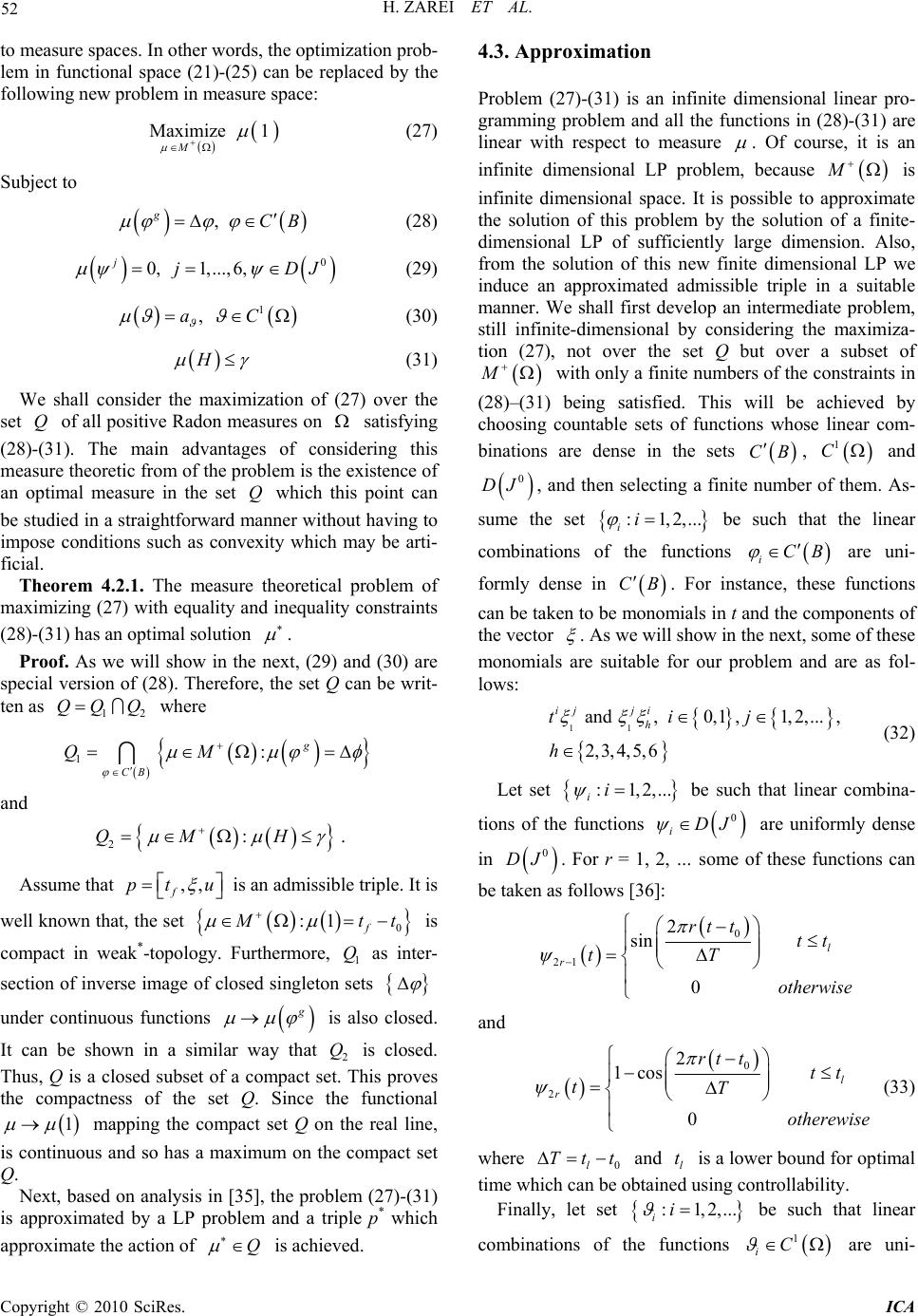

H. ZAREI ET AL.
52
to measure spaces. In other words, the optimization prob-
lem in functional space (21)-(25) can be replaced by the
following new problem in measure space:


Maximize 1
M 

 (27)
Subject to


,
gCB
 

  (28)
 
0
0, 1,...,6,
jjDJ
   (29)
 
1
,aC

   (30)

H



(31)
We shall consider the maximization of (27) over the
set Q of all positive Radon measures on  satisfying
(28)-(31). The main advantages of considering this
measure theoretic from of the problem is the existence of
an optimal measure in the set Q which this point can
be studied in a straightforward manner without having to
impose conditions such as convexity which may be arti-
ficial.
Theorem 4.2.1. The measure theoretical problem of
maximizing (27) with equality and inequality constraints
(28)-(31) has an optimal solution

.
Proof. As we will show in the next, (29) and (30) are
special version of (28). Therefore, the set Q can be writ-
ten as 12
QQ Q where




1:g
CB
QM







and
 

2:QM H


 .
Assume that ,,
f
pt u



is an admissible triple. It is
well known that, the set
 

0
:1 f
M
tt 

  is
compact in weak*-topology. Furthermore, 1 Q as inter-
section of inverse image of closed singleton sets




under continuous functions

g

 is also closed.
It can be shown in a similar way that 2 Q is closed.
Thus, Q is a closed subset of a compact set. This proves
the compactness of the set Q. Since the functional

1   mapping the compact set Q on the real line,
is continuous and so has a maximum on the compact set
Q.
Next, based on analysis in [35], the problem (27)-(31)
is approximated by a LP problem and a triple p* which
approximate the action of Q 


is achieved.
4.3. Approximation
Problem (27)-(31) is an infinite dimensional linear pro-
gramming problem and all the functions in (28)-(31) are
linear with respect to measure

. Of course, it is an
infinite dimensional LP problem, because


M


is
infinite dimensional space. It is possible to approximate
the solution of this problem by the solution of a finite-
dimensional LP of sufficiently large dimension. Also,
from the solution of this new finite dimensional LP we
induce an approximated admissible triple in a suitable
manner. We shall first develop an intermediate problem,
still infinite-dimensional by considering the maximiza-
tion (27), not over the set Q but over a subset of


M


with only a finite numbers of the constraints in
(28)–(31) being satisfied. This will be achieved by
choosing countable sets of functions whose linear com-
binations are dense in the sets

CB
,


1
C

and


0
DJ , and then selecting a finite number of them. As-
sume the set


:1,2,...
ii
  be such that the linear
combinations of the functions

iCB


 are uni-
formly dense in


CB
. For instance, these functions
can be taken to be monomials in t and the components of
the vector

. As we will show in the next, some of these
monomials are suitable for our problem and are as fol-
lows:
 

11
and ,0,1,1,2,...,
2,3, 4,5, 6
ij ji
h
tij
h
 
 (32)
Let set


:1,2,...
ii
  be such that linear combina-
tions of the functions

0
iDJ
  are uniformly dense
in


0
DJ . For r = 1, 2, … some of these functions can
be taken as follows [36]:


0
21
2
sin
0
l
r
rt ttt
tT
otherwise











and


0
2
2
1cos
0
l
r
rt ttt
tT
otherewise











(33)
where 0l
Ttt

 and l t is a lower bound for optimal
time which can be obtained using controllability.
Finally, let set


:1,2,...
ii
  be such that linear
combinations of the functions

1
iC
  are uni-

H. ZAREI ET AL.
53
formly dense in

1
C. These functions can be consid-
ered monomials in t as follows:
(),0,1,2...
s
stts
  (34)
Remark 1. With respect to (15) and (17) it can be seen
that (29) and (30) are also achieved from (28) by setting
   
,j ttt t
 
 and
  
0
,t tt d

  re-
spectively.
The first approximation will be completed by using
above subjects and the following propositions.
Proposition 4.3.1. Consider the linear program con-
sisting of the maximizing function

1   over the
set
M
Q of measures in


M

satisfying:

,1,,
g
ii
iM    

H



Then max (1)
M
MQ
  tends to max (1)
Q

 as
M →∞.
Proof. We have 12M QQ QQ ; hence,
12 . M

    Therefore, {}
n

is non
increasing and bounded sequence then converges to a
number

such that

 . We show that,



.
Set
1
M
M
RQ


. Then, RQ and max (1)
R

. It
is sufficient to show RQ. Assume R


and
()CB


. Since Linear combinations of the functions

,1,2,...
jj
  are uniformly dense in

CB
, there is
the Sequence


,1,2,...
kj
span j  
 such that k


tends to

uniformly as k→∞. Hence, 1
S, 2
S and 3
S
tend to zero as k→∞ where 1sup k S




,
2sup t tk
S


 and 3sup k
S

 
. We have
R

, and functional


f
f   is linear. Therefore,

g
kk



and
 
 


 



123
,,,,
,,
,, 2
t
ggg
kk
k
tk k
ttgtu
ttd
SgtudSd S





 
 


 




 







Since the right-hand side of the above inequality tends
to zero as k→∞, while left-hand side is independent of
k, therefore ()
g

  . Thus RQ and



which implies



.
Proposition 4.3.2. The measure

 in the set
M
Q at
which the functional (1)

  attains its maximum has
the form
1
1
()
M
j
j
j
z 




 (35)
where 0,
jj
z 

 and )(z

is unitary atomic meas-
ure with the support being the singleton set {}
j
z

, charac-
terized by()( )(),zFFz z


.
Proof. See appendix of [35].
Therefore, with respect to above descriptions we re-
strict our attention to finding measure in form


1
1()
M
j
j
jz



, which maximizes functional


1

 
and satisfies in (31) and M number of constraints in the
form of (28)-(30). Clearly, 1
1
()( ),
M
jj
j
F
FzF 




()C

. Therefore, by choosing 1
M
number of functions
in the form of (32), S number of functions in the form of
(34) and 2
M

number of functions in the form of (33),
which leads to 22 6
M
M


number of functions of the
type (17) where are numbered sequentially as ,
h

2
1,...,hM

, infinite dimensional problem (27)-(31) is
approximated with following finite dimensional nonlin-
ear programming (NLP) problem:

1
0, 1
Maximize
jj
M
j
zM j 



 
 (36)
Subject to

1
1
1
, 1,...,
Mg
ji ji
j
ziM  


 
 (37)

1
2
1
0, 1,...,
M
jh j
j
zhM 



 (38)

1
1
,1,,
M
js j
j
zas S





 (39)

1
1
M
jj
j
Hz





 (40)
where, 12
M
MM S

. We confront with NLP with
more than 2( 1)M

unknowns
j

, ,1,...,1
j
zj M.
Finally, the following proposition enables us to approxi-
mate the problem via the finite dimensional linear pro-
gramming problem.
Proposition 4.3.3. Let

12
, ,...,
N
N
y
yy be a cou-
ntable dense subset of

, for any N sufficiently large
number. Given 0

, a measure ()vM

 can be

H. ZAREI ET AL.
54
found such that:

1
1,...,
gg
ii
viM  

 (41)

2
1,...,
hh
vhM  

 (42)
 
1,...,
ss
vsS 


(43)
 
vH H



 (44)
where measure v has the form

1
1
M
jj
j
vz 


 (45)
where the coefficients ,1,...,1
jjM

 are the same as
optimal measure (35), and zj ΩN, j = 1,…, M + 1.
Proof. We rename functions
g
i

’s, h

’s,
s
v’s and
H
sequentially as ,1,2,..., 1
j
fj M. Then, for j = 1,…,
M + 1,
 



1
1
1
,
1
max
M
jijiji
i
M
ijiji
ij
i
vff zf z
fz fz









 








.
j
f
’s are continues. Therefore, , max
ij can be made less
than 1
1
M
j
j




 by choosing ,1,2,..., 1
i
zi M, suffi-
ciently near to i z.
For construction of dense subset
N
, J is divided to S
subintervals as follows:

00
1,,1,2,...,1
11
s
sTsT
Jtts S
SS


 



and

,
Slf
J
tt

 (46)
Furthermore, intervals Ai’s and Uj’s are divided into ni
and mj subintervals respectively, then the set Ω is divided
into N = Sn1 n2 n3 n4 n5 m1 m2 cells. One point is chosen
from each cell. In this way we will have a grid of points,
which are numbered sequentially as j y1 (, ,...,
j
j
t

6,, )
j
jj
PR
uu

, j = 1,…, N.
Remark 2. It is well known that each function type
(34) can be approximated in a nice way by a linear com-
bination of characteristic function of subintervals of J. In
practice we consider ()(), 1,...,
s
sJ
ttsS   instead of
functions of the type (34), where
s
J
’s are given by (46)
and
s
J

denotes the characteristic function of
s
J
. The
main reason for this choice of
s

’s is related to their
essential role in construction of control functions. For
more details see [35,36].
Considering (45) the NLP (36)-(40) is converted to the
following LP:
01
Maximize
j
N
j
j



 (47)
subject to

1
1
, 1,...,
Ng
ji ji
j
yiM  

 
 (48)

2
1
0, 1,...,
N
jh j
j
yhM 


 (49)

1
N
jj
j
Hy




 (50)



1
1
21
11
1
1
l
j
j
Sl
j
jSl
Sl
j
fl
jS l
T
S
T
S
tt





 











(51)


, 2,3,4,5,6
if i
tAi   (52)
where N
lS

. Of course, we need only to construct the
function (.)u, since the (.)

is simply the corresponding
solution of differential Equations (1)-(6) which can be
estimated numericall. Using simplex method, nonzero
optimal solution 12
,,,
p
ii i




, 12
p
ii i  of LP
(47)-(52) can be found where p cannot exceed the num-
ber of constraints i.e., 12 1pM MS

.
Setting 00it



, piecewise control pair

() ()
P
utu t,

()
R
ut which approximate the action of the optimal con-
trol, is constructed based on these nonzero coefficients as
follows [35,36]:


1
00
,,
,1,2,...,
0
iii i
jjh h
jj
PR
hh
uu t
utj p
otherewise












It should be remembered, i
j
P
u and i
j
R
u are respec-
tively 7th and 8th components of
j
i
y.

H. ZAREI ET AL.
55
5. Numerical Results
In our implementation, we set 114M and chosen func-
tions

from


CB
 are as follows:
11
22
12 3 4 5 611213141516
,,,,,,,,, ,, ,,tt
 
Furthermore, we set 22M. Hence, we have 212M

number of functions in the form of (17). Parameter S is
set to 11 and desired lower bound for optimal time is set
to 2007.5(5.5)
l
t years. Setting (0,0)u, and solv-
ing ODE (1)-(6) using 4th order Runge-Kutta method,
shows that at 0620t,

0(350,12.40,1.26,0.16,t
 
18454) . Starting points of our simulation runs are:
x(0) = 103 cellsµl-1, v(0) = 104 copiesml-1, y(0) = 0
cellsµl-1, w(0) = 10-3 cellsml-1, z(0) = 10-7cellsµl-1 and
r(0) = 2 × 10-7 mlcopies-1day-1.
Maximum values for uP and uR, are 0.7 and 9 × 10-10
respectively [7]. Therefore, the coefficient

for balanc-
ing both PI and RTI costs in (8) is set to


2
-10
0.7
910




. Furthermore, the total costs are bounded
above by 480

. By using controllability, considered
ranges for states and controls and corresponding parti-
tions for construction of yj, j=1,…, N are summarized in
Table 2. Note that, selected values from the set U1 for
construction of yj’s are 0, 0.4 and 0.7. These values indi-
cate off, moderate and strong PI-therapy. Similarly, cor-
responding values for RTI control are 0, 5 × 10-10 and 9 ×
10-10 [7]. Therefore, we have linear programming with
M = 33 constraints and N = 59405 unknowns, that is
solved using simplex method and environment of MAT-
LAB. Implementing the corresponding LP model, the sub-
optimal time has been found 2133.2 (71.11)
f
tMonths
.
Figure 1 shows the resulting suboptimal control pair.
The response of the system to the control functions is
depicted in Figure 2. Figure 2(a) shows that condition
(14) violates in a subinterval of J, which is due to ap-
proximate nature of control pair and can be ignored. Be-
cause, the length of this subinterval is very small as
compared to the length of J. We found 1( )199.28
f
t 
,
which is close to exact value i.e., 200. From Figures 2(a)
and 2(b), we see drop in the number of CD4+ T-cells,
and a rise in viral load following the initial infection until
about the third month. After this time, CD4+ T-cells start
recovering and virus starts decreasing due to the immune
response, but can never eradicate virus completely. Then
CD4+ T-cells level decreases and viral load increases
due to de struction of immune system in absence of
treatment. Figures 2(b) and 2(c) show a clear correlation
between the CTLe and virus population. As the virus
increases upon initial infection, CTLe increases in order
to decrease the virus. Once this is accomplished, virus
decreases. Then virus grows back slowly, and this trig-
gers an increase in the CTLe population. CTLe, further
increases in an attempt to keep the virus at constant lev-
els but lose the battle because of virus-induced impair-
ment of CD4+ T-cell function, in absence of treatment
(dotted line). Memory CTL responses depend on the
Table 2. Considered ranges for states and controls and cor-
responding number of partitions.
State Range Number of partitions
1

A1 = [200, 1000] n
1 = 5
2

A2 = [5, 30] n
2 = 3
3

A3 = [0, 1.6] n
3 = 2
4

A4 = [0, 1.3] n
4 = 2
5

A5 = [500, 35000] n
5 = 10
6

A6 = [0, 2 × 10-7] n
6 = 1
P
u U1 = [0, 0.7] m
1 = 3
R
u U2 = [0, 9 × 10-10] m
2 = 3
Figure 1. The suboptimal piecewise constant control pair (.)
P
u and (.)
R
u.

H. ZAREI ET AL.
56
(a) (b)
(c) (d)
Figure 2. Dynamic behavior of the state variables x, v, w and z versus time in the case of untreated (dotted line) and treated
infected patients (solid line).
presence of CD4+ T-cell help. Figures 2(a) and 2(b)
show that, in presence of treatment the virus is controlled
to very low levels and CD4+ T-cells are maintained
above the critical levels for relatively long time. There-
fore, immune response expands for relatively long time
successfully. Furthermore, these figures indicate inverse-
coloration between viral load and CD4+ T-cells level.
From Figures 2(c) and 2(d) interestingly, a decrease in
CTL’s occurs in response to therapy can be observed.
The extent of the decrease is directly correlated with the
increase in treatment effectiveness which is consistent
with experimental findings [37].
6. Conclusions
In this paper, we considered a system of ordinary differ-
ential equations, which describe various aspects of the
interaction of HIV with healthy cells in fast progressive
patient, for constructing a time optimal control problem
which maximizes asymptomatic stage of patient. A
measure theoretical method is used to solve such kind of
problems, and numerical results, confirmed the effec-
tiveness of this approach.
7. References
[1] T. W. Chun, L. Stuyver, S. B. Mizell, L. A. Ehler, J. A.
Mican, M. Baseler, A. L. Lloyd, M. A. Nowak and A. S.
Fauci, “Presence of an Inducible HIV-1 Latent Reservoir
During Highly Active Antiretroviral Therapy,” Proceed-
ings of the National Academy of Sciences, Vol. 94, No.
24, 1997, pp. 13193-13197.
[2] D. Finzi, M. Hermankova, T. Pierson, L. M. Carruth, C.

H. ZAREI ET AL.
57
Buck, R. E. Chaisson, T. C. Quinn, K. Chadwick, J.
Margolick, R. Brookmeyer, et al., “Identification of a
Reservoir for HIV-1 in Patients on Highly Active Anti-
retroviral Therapy,” Sci ence , Vol. 278, No. 5341, 1997,
pp. 1295-1300
[3] J. K. Wong, M. Hezareh, H. F. Gunthard, D. V. Havlir, C.
C. Ignacio, C. A. Spina and D. D. Richman, “Recovery of
Replication-Competent HIV Despite Prolonged Suppres-
sion of Plasma Viremia,” Scienc e, Vol. 278, No. 5341,
1997, pp. 1291-1295.
[4] M. M. Hadjiandreou, R. Conejeros and V. S. Vassiliadis,
“Towards a Long-Term Model Construction for the Dy-
namic Simulation of HIV Infection,” Mathematical Bio-
sciences and Engineering, Vol. 4, No. 3, 2007, pp. 489-
504.
[5] A. S. Perelson, A. U. Neumann, M. Markowitz, et al.,
“HIV-1 Dynamics in Vivo: Virion Clearance Rate, In-
fected Cell Life-Span, and Viral Generation Time,” Sci-
ence, Vol. 271, No. 5255, 1996, pp. 1582-1586.
[6] D. Wodarz and M. A. Nowak, “Specific Therapy Re-
gimes Could Lead to Long-Term Immunological Control
of HIV,” Proceedings of the National Academy of Sci-
ences, Vol. 96, No. 6, 1999, pp. 14464-14469.
[7] A. Landi, A. Mazzoldi, C. Andreoni, M. Bianchi, A.
Cavallini, M. Laurino, L. Ricotti, R. Iuliano, B. Matteoli
and L. Ceccherini-Nelli, “Modelling and Control of HIV
Dynamics,” Computer Methods and Programs in Bio-
medicine, Vol. 89, No. 2, 2008, pp. 162-168.
[8] K. R. Fister, S. Lenhart and J. S. McNally, “Optimizing
Chemotherapy in an HIV Model,” Electronic Journal of
Differential Equations, Vol. 1998, No. 32, 1998, pp. 1-
12.
[9] M. M. Hadjiandreou, R. Conejeros and D. I. Wilson,
“Long-Term HIV Dynamics Subject to Continuous The-
rapy and Structured Treatment Interruptions,” Chemical
Engineering Science, Vol. 64, No. 7, 2009, pp. 1600-
1617.
[10] W. Garira, D. S. Musekwa and T. Shiri, “Optimal Control
of Combined Therapy in a Single Strain HIV-1 Model,”
Electronic Journal of Differential Equations, Vol. 2005,
No. 52, 2005, pp. 1-22.
[11] J. Karrakchou, M. Rachik and S. Gourari, “Optimal Con-
trol and Infectiology: Application to an HIV/AIDS
Model,” Journal of Applied Mathematics and Computing,
Vol. 177, No. 2, 2006, pp. 807-818.
[12] A. Heydari, M. H. Farahi and A. A. Heydari, “Chemo-
therapy in an HIV Model by a Pair of Optimal Control,”
Proceedings of the 7th WSEAS International Conference
on Simulation, Modelling and Optimization, Beijing,
2007, pp. 58-63.
[13] B. M. Adams, H. T. Banks, H. D. Kwon and H. T. Tran,
“Dynamic Multidrug Therapies for HIV: Optimal and
STI Control Approaches,” Mathematical Biosciences and
Engineering, Vol. 1, No. 2, 2004, pp. 223-241.
[14] F. Neri, J. Toivanen and R. A. E. Mäkinen, “An Adaptive
Evolutionary Algorithm with Intelligent Mutation Local
Searchers for Designing Multidrug Therapies for HIV,”
Applied Intelligence, Vol. 27, No. 3, 2007, pp. 219-235.
[15] R. Culshaw, S. Ruan and R. J. Spiteri, “Optimal HIV
Treatment by Maximizing Immune Response,” Journal of
Mathematical Biology, Vol. 48, No. 5, 2004, pp. 545-562.
[16] O. Krakovska and L. M. Wahl, “Costs Versus Benefits:
Best Possible and Best Practical Treatment Regimens for
HIV,” Journal of Mathematical Biology, Vol. 54, No. 3,
2007, pp. 385-406.
[17] C. D. Myburgh and K. H. Wong, “An Optimal Control
Approach to Therapeutic Intervention in HIV Infected
Individuals,” Proceedings of the Third International Con-
ference on Control Theory and Applications, Pretoria,
South Africa, 2001.
[18] B. M. Adams, H. T. Banks, M. Davidian, H. D. Kwon, H.
T. Tran, S. N. Wynne and E. S. Rosenberg, “HIV Dy-
namics: Modeling, Data Analysis, and Optimal Treatment
Protocols,” Journal of Computational and Applied Math-
ematics, Vol. 184, No. 1, 2005, pp. 10-49.
[19] J. Alvarez-Ramirez, M. Meraz and J. X. Velasco-Her-
nandez, “Feedback Control of the Chemotherapy of
HIV,” International Journal of Bifurcation and Chaos,
Vol. 10, No. 9, 2000, pp. 2207-2219.
[20] S. Butler, D. Kirschner and S. Lenhart, “Optimal Control
of Chemotherapy Affecting the Infectivity of HIV,” In: O.
Arino, D. Axelrod, M. Kimmel and M. Langlais, Eds.,
Advances in Mathematical Population Dynamics: Mole-
cules, Cells, Man, World Scientific, Singapore, pp.104-
120.
[21] H. Shim, S. J. Han, C. C. Chung, S. Nam and J. H. Seo,
“Optimal Scheduling of Drug Treatment for HIV Infec-
tion: Continuous dose Control and Receding Horizon
Control,” International Journal of Control, Automation,
and Systems, Vol. 1, No. 3, 2003, pp. 401-407.
[22] D. Kirschner, S. Lenhart and S. Serbin, “Optimal Control
of the Chemotherapy of HIV Infection: Scheduling,
Amounts and Initiation of Treatment,” Journal of
Mathematical Biology, Vol. 35, No. 7, 1997, pp. 775-792.
[23] U. Ledzewicz and H. Schättler, “On Optimal Controls for
a General Mathematical Model for Chemotherapy of
HIV,” Proceedings of the 2002 American Control Con-
ference, Anchorage, Vol. 5, 2002, pp. 3454-3459.
[24] R. Zurakowski, M. J. Messina, S. E. Tuna and A. R. Teel,
“HIV Treatment Scheduling Via Robust Nonlinear Model
Predictive Control,” Proceedings of the 5th Asian Control
Conference, Melbourne, Vol. 1, 2004, pp. 25-32.
[25] R. Zurakowski and A. R. Teel, “Enhancing Immune Re-
sponse to HIV Infection Using MPC-Based Treatment
Scheduling,” Proceedings of the 2003 American Control
Conference, Denver, Vol. 2, 2003, pp. 1182-1187.
[26] R. Zurakowski, A. R. Teel and D. Wodarz, “Utilizing
Alternate Target Cells in Treating HIV Infection through
Scheduled Treatment Interruptions,” Proceedings of the
2004 American Control Conference, Melbourne, Vol. 1,
2004, pp. 946-951.
[27] R. Zurakowski and A. R. Teel, “A Model Predictive Con-
trol Based Scheduling Method for HIV Therapy,” Jour-
nal of Theoretical Biology, Vol. 238, No. 2, 2006, pp.
368-382.
[28] H. T. Banks, H. D. Kwon, J. Toivanen and H. T. Tran,

H. ZAREI ET AL.
58
“An State Dependent Riccati Equation Based Estimator
Approach for HIV Feedback Control,” Optimal Control
Applications and Methods, Vol. 27, No. 2, 2006, pp. 93-
121.
[29] M. A. L. Caetano and T. Yoneyama, “Short and Long
Period Optimization of Drug Doses in the Treatment of
AIDS,” Anais da Academia Brasileira de Ciências, Vol.
74, No. 3, 2002, pp. 379-392.
[30] A. M. Jeffrey, X. Xia and I. K. Craig, “When to Initiate
HIV Therapy: A Control Theoretic Approach,” IEEE
Transactions on Biomedical Engineering, Vol. 50, No. 11,
2003, pp. 1213-1220.
[31] J. J. Kutch, P. Gurfil, “Optimal Control of HIV Infection
with a Continuously-Mutating Viral Population,” Pro-
ceedings of the 2002 American Control Conference, An-
chorage, Vol. 5, 2002, pp. 4033-4038.
[32] P. Borrow, A. Tishon, S. Lee, J. Xu, I. S. Grewal, M. B.
Oldstone and R. A. Flavell, “CD40L-Deficient Mice
Show Deficits in Antiviral Immunity and Have an Im-
Paired Memory CD8 CTL,” Journal of Experimental
Medicine, Vol. 183, No. 5, 1996, pp. 2129-2142.
[33] C. Young, “Calculus of Variations and Optimal Control
Theory,” Sunders, Philadelphia, 1969.
[34] D. A. Wilson and J. E. Rubio, “Existence of Optimal
Controls for the Diffusion Equation,” Journal of Optimi-
zation Theory and Applications, Vol. 22, 1977, pp. 91-
101.
[35] J. E. Rubio, “Control and Optimization: The Linear
Treatment of Non-linear Problems,” Manchester Univer-
sity Press, Manchester, 1986.
[36] H. H. Mehne, M. H. Farahi and A. V. Kamyad, “MILP
Modelling for the Time Optimal Control Problem in The
Case of Multiple Targets,” Optimal Control Applications
and Methods, Vol. 27, No. 2, 2005, pp. 77-91.
[37] X. Jin, et al., “An Antigenic Threshold for Maintaining
Human Immunodeficiency Virus Type 1-Specific Cyto-
toxic T Lymphocytes,” Molecular Medicine, Vol. 6, 2000,
pp. 803-809.