Paper Menu >>
Journal Menu >>
 J. Software Engineering & Applications, 2010, 3, 746-755 doi:10.4236/jsea.2010.38086 Published Online August 2010 (http://www.SciRP.org/journal/jsea) Copyright © 2010 SciRes. JSEA A Residual Time Based Scheduling: Performance Modeling in M/G/C Queueing Applications* Sarah Tasneem1, Lester Lipsky2, Reda Ammar2, Howard Sholl2 1Math and Computer Science, Eastern Connecticut State University, Willimantic, USA; 2Computer Science and Engineering, Uni- versity of Connecticut, Storrs, USA. Email: tasneems@easternct.edu Received June 3rd 2010; revised July 16th 2010; accepted July 20th 2010. ABSTRACT It is well known, in queueing theory, that the system performance is greatly influenced by scheduling policy. No univer- sal optimum scheduling strategy exists in systems where individual customer service demands are not known a priori. However, if the distribution of job times is known, then the residual time (expected time remaining for a job), based on the service it has already received, can be calculated. Our particular research contribution is in exploring the use of this function to enhance system performance by increasing the probability that a job will meet its deadline. In a detailed discrete event simulation, we have tested many different distributions with a wide range of C2 and shapes, as well as for single and dual processor system. Results of four distributions are reported here. We compare with RR and FCFS, and find that in all distributions studied our algorithm performs best. In the study of the use of two slow servers versus one fast server, we have discovered that they provide comparable performance, and in a few cases the double server system does better. Keywords: Simulation, Residual Time Scheduling, Coefficient of Variation, M/G/C Queue, Processor Sharing 1. Introduction There have been innumerable papers written on how to optimize performance in queueing systems. They cover any number of different goals and conditions. From our point of view they fall into two categories (with many possibilities in between): 1) The service demand of each customer is known, and; 2) The service demands of the individual customers are not known, but the probability distribution function (pdf) of those de- mands is presumed to be known. So, for instance, the mean and variance, (the expectation, or mean, of the deviation squared of the variable from its expected value or mean) over all customers might be known, even though the time needed by a particular customer is not known until that customer is finished. Within each of these categories there are many pos- sible goals. For instance, the goal might be to minimize the system time, as in job processing in computer sys- tems, or minimize the waiting time, as in setting up telecommunication links. However, both of these would be useless in situations where there are critical deadlines, as would be the case in airport security lines, where it would be more important to maximize the fraction of passengers who get through in time to catch their flights, or in the case of web server where the millions of users surfing the Internet, are unwilling to spend more than few seconds waiting for a web page to be displayed. One of the major metrics to be considered for a high performance web server is the number of pages downloaded per second by a web server. In this paper we consider the second category with the goal of maximizing the number of jobs that meet their deadline. We compare several queueing disciplines for systems with Poisson customer arrivals to a service station, with a given service time distribution. The distributions we consider include: Uniform, Exponential, hyper ex- ponential and hyper-Erlangian. The distributions were chosen to show a wide range of coefficient of variation of service times (2 C) which is the ratio of the standard deviation of the service time to its mean. The numerous scheduling disciplines proposed for multiprogrammed systems, for the most part the evalu- ation has been based on workloads showing a relatively low variability in the service requirements of jobs. In other words when 21C . However, reports from va- * Partially funded by CSU-AAUP Summer Research Grant 2010- 2011 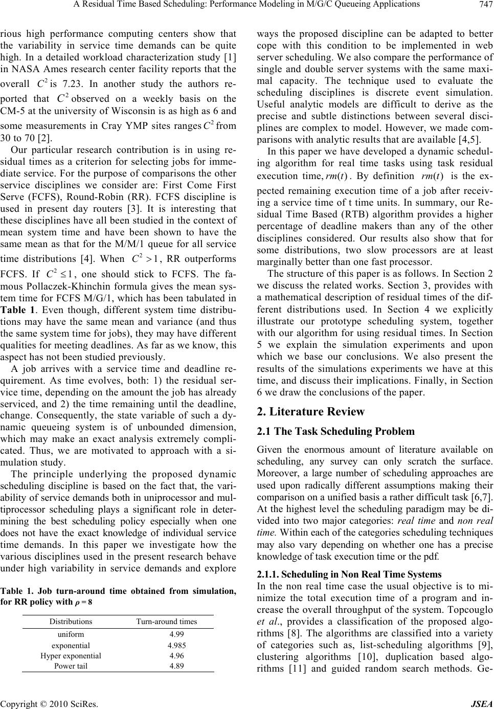 A Residual Time Based Scheduling: Performance Modeling in M/G/C Queueing Applications Copyright © 2010 SciRes. JSEA 747 rious high performance computing centers show that the variability in service time demands can be quite high. In a detailed workload characterization study [1] in NASA Ames research center facility reports that the overall 2 Cis 7.23. In another study the authors re- ported that 2 Cobserved on a weekly basis on the CM-5 at the university of Wisconsin is as high as 6 and some measurements in Cray YMP sites ranges2 Cfrom 30 to 70 [2]. Our particular research contribution is in using re- sidual times as a criterion for selecting jobs for imme- diate service. For the purpose of comparisons the other service disciplines we consider are: First Come First Serve (FCFS), Round-Robin (RR). FCFS discipline is used in present day routers [3]. It is interesting that these disciplines have all been studied in the context of mean system time and have been shown to have the same mean as that for the M/M/1 queue for all service time distributions [4]. When 21C, RR outperforms FCFS. If 21C, one should stick to FCFS. The fa- mous Pollaczek-Khinchin formula gives the mean sys- tem time for FCFS M/G/1, which has been tabulated in Table 1. Even though, different system time distribu- tions may have the same mean and variance (and thus the same system time for jobs), they may have different qualities for meeting deadlines. As far as we know, this aspect has not been studied previously. A job arrives with a service time and deadline re- quirement. As time evolves, both: 1) the residual ser- vice time, depending on the amount the job has already serviced, and 2) the time remaining until the deadline, change. Consequently, the state variable of such a dy- namic queueing system is of unbounded dimension, which may make an exact analysis extremely compli- cated. Thus, we are motivated to approach with a si- mulation study. The principle underlying the proposed dynamic scheduling discipline is based on the fact that, the vari- ability of service demands both in uniprocessor and mul- tiprocessor scheduling plays a significant role in deter- mining the best scheduling policy especially when one does not have the exact knowledge of individual service time demands. In this paper we investigate how the various disciplines used in the present research behave under high variability in service demands and explore Table 1. Job turn-around time obtained from simulation, for RR policy with=8ρ Distributions Turn-around times uniform 4.99 exponential 4.985 Hyper exponential 4.96 Power tail 4.89 ways the proposed discipline can be adapted to better cope with this condition to be implemented in web server scheduling. We also compare the performance of single and double server systems with the same maxi- mal capacity. The technique used to evaluate the scheduling disciplines is discrete event simulation. Useful analytic models are difficult to derive as the precise and subtle distinctions between several disci- plines are complex to model. However, we made com- parisons with analytic results that are available [4,5]. In this paper we have developed a dynamic schedul- ing algorithm for real time tasks using task residual execution time,()rm t. By definition ()rm t is the ex- pected remaining execution time of a job after receiv- ing a service time of t time units. In summary, our Re- sidual Time Based (RTB) algorithm provides a higher percentage of deadline makers than any of the other disciplines considered. Our results also show that for some distributions, two slow processors are at least marginally better than one fast processor. The structure of this paper is as follows. In Section 2 we discuss the related works. Section 3, provides with a mathematical description of residual times of the dif- ferent distributions used. In Section 4 we explicitly illustrate our prototype scheduling system, together with our algorithm for using residual times. In Section 5 we explain the simulation experiments and upon which we base our conclusions. We also present the results of the simulations experiments we have at this time, and discuss their implications. Finally, in Section 6 we draw the conclusions of the paper. 2. Literature Review 2.1 The Task Scheduling Problem Given the enormous amount of literature available on scheduling, any survey can only scratch the surface. Moreover, a large number of scheduling approaches are used upon radically different assumptions making their comparison on a unified basis a rather difficult task [6,7]. At the highest level the scheduling paradigm may be di- vided into two major categories: real time and non real time. Within each of the categories scheduling techniques may also vary depending on whether one has a precise knowledge of task execution time or the pdf. 2.1.1. Scheduling in Non Real Time Systems In the non real time case the usual objective is to mi- nimize the total execution time of a program and in- crease the overall throughput of the system. Topcouglo et al., provides a classification of the proposed algo- rithms [8]. The algorithms are classified into a variety of categories such as, list-scheduling algorithms [9], clustering algorithms [10], duplication based algo- rithms [11] and guided random search methods. Ge-  A Residual Time Based Scheduling: Performance Modeling in M/G/C Queueing Applications Copyright © 2010 SciRes. JSEA 748 netic Algorithms (GAs) [12] are one of the widely stu- died guided random search techniques for the task scheduling problem. Although they provide a good quality of schedules, the execution time of Genetic Algorithms is significantly higher than the other alter- natives. Several researchers have studied the problem of scheduling, which is known to be NP-complete in its general form, when the program is represented as a task graph [8]. The execution time of any task and the communication cost between any pair of processors is considered to be one time unit. Thus, they have con- sidered only deterministic execution time. Adam et al. [13] studied both deterministic and stochastic models for task execution time and made a comparison of dif- ferent list scheduling algorithms. For the latter, task execution is limited to the uniform distribution. Kwok and Ahmed [9] focused on taxonomy of DAG sched- uling algorithms based on a static scheduling problem, and are therefore only partial. Some algorithms assume the computational cost of all the tasks to be uniform. This simplifying assumption may not hold in practical situations. It is not always realistic to assume that the task execution times are uniform. Because the amount of computations encapsulated in tasks are usually var- ied. Others do not specify any distribution for task execution time. They just assume any arbitrary value. 2.1.2. Scheduling in Real Time Systems Scheduling algorithm in RT applications can be classi- fied along many dimensions. For example: periodic tasks, pre-emptable non-pre-emptable. Some of them deal only with periodic tasks while others are intended only for a-periodic tasks. Another possible classifica- tion ranges from static to dynamic. Ramamaritham and Stankovic [14] discuss several task scheduling para- digms and identify several classes of scheduling algo- rithms. A majority of scheduling algorithms reported in the literature, perform static scheduling and hence have limited applicability since not all task characteristics are known a priori and further tasks arrive dynamically. Recently many scheduling algorithms [15] have been proposed to dynamically schedule a set of tasks with computation times, deadlines, and task requirements. Each task is characterized by its worst-case computa- tion time deadline, arrival time and ready time. Ramamritham in [16] discusses a static algorithm for allocating and scheduling subtasks of periodic tasks across sites in distributed systems. The computation times of subtasks represent the worst-case computation time and are considered to be uniformly distributed between a minimum (50 time unit) and maximum (100 time unit) value. It is assumed that the execution of each subtask cannot be preempted. This way of select- ing the execution time range (from 50 to 100) reduces C2 to a very small value (= 4/27), which the authors may not have realized. Chetto and Chetto [17] consid- ered the problem of scheduling hard periodic real time tasks and hard sporadic tasks (tasks that arrive are re- quired to be run just once [14]). In addition to compu- tation time and period, each periodic task is character- ized by its dynamic remaining execution time. But the authors have not mentioned how to obtain the remain- ing execution time in a dynamic manner. Liu and Lay- land [18] were perhaps the first to formally study pri- ority driven algorithms. They focused on the problem of scheduling periodic tasks on a single processor and proposed two preemptive algorithms. The first one is called Rate-Monotonic (RM) algorithm, which assigns static priorities to periodic tasks based on their periods. The second one is called the Earliest Deadlines First (EDF), a dynamic priority assignment algorithm. The closer a tasks’ deadline, the higher the priority. This again is an intuitive priority assignment policy. EDF and RM schedulers do not provide any quality of ser- vice (QoS) guarantee when the system is overloaded by overbooking. Since, EDF [18] does not make use of the execution time of tasks, it is difficult to mix non-real- time and real-time tasks effectively. Scheduling both real-time and non real-time tasks under load requires knowing how long a real-time task is going to run. As a result, some new/different scheduling approach that addresses these limitations is desirable. One can de- termine the latest time the task must start executing if one has the knowledge of the exact time of how long a task will run. Thus, the scheduler may delay a job to start executing in order to increase the number of jobs meeting deadlines. In this paper, we investigated this issue and developed a dynamic scheduling strategy, which includes both the deadline and the estimated execution time. For dynamic scheduling with more than one proces- sor, Mok and Destouzos [19] show that an optimal scheduling algorithm does not exist. These negative results point out the need for new approaches to solve scheduling problems in such systems. Those ap- proaches may be different depending on the job service time distribution (job size variability). In this paper we have addressed this issue by running simulation ex- periments for several distributions for both single and multiple processor systems. 3. Terminology and Mathematical Background In this section we first define the job execution model. Then we present the mathematical expressions for resid- ual times for different job service time distributions. Let X be the job execution time which can be modeled either by deterministic or stochastic distribution. In the present paper, we consider the latter. Task execution time can follow any standard distribution, for example: uniform, exponential, hyper exponential, etc, or take discrete val-  A Residual Time Based Scheduling: Performance Modeling in M/G/C Queueing Applications Copyright © 2010 SciRes. JSEA 749 ues with associated probabilities. Before that we show the well-known Pollaczek- Khinchin formula, as 22 1 11 2 C n which states that the mean number of jobs in a system, n de- pends only on their arrival rate , the mean, []EX and variance 2 of the service time distribution. In the for- mula it is expressed in terms of the coefficient of varia- tion 22 2 /( [])CEX . 3.1 Job Execution Model We assume that job arrival follows a Poisson process. Tasks are independent and identically distributed and preemptable. Each job is characterized by the follow- ing: task arrival time i A , task execution time i Etask deadline i D, task start time, i S. A job is ready to exe- cute as soon as it arrives, regardless of processor availability. Tasks may have to wait for some time, i W, before they start executing for the first time due to scheduling decision. As a result, we haveiii SAW , where 0 i W. By definition, the Cumulative Distribution Function (CDF) is, 0 () ()(). x F xPXx fxdx . The Reli- ability function, () ()(). x RxPXxfx dx where ()() 1Rx Fx. The expected execution time, 0 0 0 () ().()Exxf xdxRxdx . The conditional reli- ability, () t Rx, is the probability that the task executes for an additional interval of duration of x given that it has already executed for time t, ()()/ () t RxRt x Rt . By definition, the task residual time [20]()rm t given that the task has already executed for t time units is; 0 ()( ()/())rm tR txR tdx . Here we show different expressions for residual time for different types of dis- tributions. Uniform: Here the task execution time follows the uniform distribution with CDF,() 2 x Fx T . The reli- ability function,2 () 2 Tx Rx T and21/3C. The resi- dual time, after time t is () (2)/2rm tt . Exponential: Here the task execution time follows the exponential distribution with CDF ()1 x F xe . The reliability function, () x Rx e .The expected value, 1 ()Ex and 21C Where, 1 is referred to as the mean service time. The residual time at time t can be shown to be equal to 1 ()rm t . Due to the memory-less property of exponential distributions the residual time, does not change with time. Hyper Exponential: In this paper we have consid- ered a two stage hyper-exponential distribution with CDF 12 12 () 1 x x Fxpe pe and 21 1pp . The reliability function 12 12 () x x Rx pepe . There are three free parameters, namely1 p, 1 and2 , where 1/ ii T . Now, we define the free parameters [5] 2 (1) 2 C and 12 2 1 pC ,121 (1/)Txp p and 212 (1/ )Txp p . Hyper exponential distribution can be used when it or desired that 21C. The resid- ual time can be shown to be 12 12 // 112 2 // 12 () tT tT tT tT pTep T e rm tpe pe Hyper Erlangian: We have considered a four stage Hyper Erlangian distribution with pdf, 11 () [fx p 12 1222 ()][()] x x xe pxe and CDF, () F x 12 112 2 1(1 )(1) x x pxep xe . The reliability function 1 11 ()(1) x Rx pxe 2 22 (1 ) x pxe . There are three free parameters, namely 1 p, 1 and 2 , where1/ ii T . For the defi- nition of those parameters we refer [5]. Hyper Erlan- gian distributions can be used when it is expected that 21C. The residual time can be shown to be ()rm t 12 12 // 1112 22 // 112 2 [2/ ][2/] (11/)(11/) tT tT tT tT pTtT epTtTe pTep Te In this case the residual time at first decreases, then increases greatly and then decreases gradually to 12 max ,TT . 4. The Scheduling Model Each process or task or job is associated with an execu- tion time. Figure 1 shows the schematic for the present Figure 1. The Scheduling Model terminating Arrival pool scheduler Current pool Job arrival  A Residual Time Based Scheduling: Performance Modeling in M/G/C Queueing Applications Copyright © 2010 SciRes. JSEA 750 scheduling model. Upon arrival, a task joins the arrival pool. The duration of those execution times of the proc- esses are not known in advance. We assume they follow a distribution function, which can either be deterministic or non-deterministic. A task will have a deadline that repre- sents a soft timing constraint on the completion of the task. The scheduler will pick a process to execute from the arrival pool depending on the scheduling policy. A proc- ess joins the current pool as soon as it is picked by the scheduler to run. Note, the CPU/s is/are being shared by several concurrent processes/tasks. The current pool keeps the record of execution time already taken of the chosen tasks (concurrent tasks). Once picked, each task i will execute for a time slice called time quantum, i q. At the end of time : i q. 1) the executing task is either completed or partially executed. A partially executed task goes back to the cur- rent pool, whereas, a completed task leaves the current pool. 2) the scheduler then chooses the next task either from the arrival pool or the current pool. We define a function called risk factor (rf). As soon as a process istarts executing, time starts running out be- fore it reaches deadline. At clock time T Cthe time left before deadline is iT DC. Let ()rm t be the re- maining execution time required to finish the given process I, which has to fit in time interval to meet the deadline. Let us define the risk factor for process i as follows: () ()/() iTi rftrm tDCA. In other words, residual time rf remainingtime before deadline 4.1 RTB Algorithm We propose a dynamic scheduling algorithm called Re- sidual Time Based (RTB) which incorporates the task residual time. Task risk factor is used as a measure to choose the next task to execute. Tasks in the task set are maintained in the order of decreasing risk factor. The proposed Residual Time Based (RTB) algorithm: 1) As soon as a job arrives. a) compute estimated residual time for the job. b) compute risk factor (rf) for the job. c) append the job to the queue. 2) Select the job that has the highest rf and execute it for the next quantum. a) compute the end time if the job is complete at or before the end of quantum. 3) At the end of each quantum. a) compute estimated residual time for each job in the queue. b) compute rf for each job in the queue. The risk factor is inversely proportional to the differ- ence between task deadline and the clock time. The risk factor increases as the task approaches to its deadline. As soon as the clock time passes the deadline the rf becomes negative if the task has not yet been completed. The goal in the present research is to increase the number of tasks meeting the deadline. As the clock time passes the dead- line the task is considered to be less important compared to tasks that are very close to deadline but have not yet crossed the deadline. Therefore, tasks with positive risk factor are given higher priority than tasks with negative risk factor. 4.2 Why does RTB Bring Enhancement The Let us consider the P-K formula from Section 3. When 21C 1 n . When21C 1 n . When 21C 1 n and FCFS gives the least wait- ing time. However, as 2 C tends to increase beyond 1, the number of jobs, n keeps on increasing over1 . So it is unwise to use FCFS. Mean number of jobs in a queue, n, for PS is 1 which is the same as M/M/1 queue. In practice, PS is implemented by RR with finite time slicing. In RR jobs form a queue upon arrival and the server picks one after another from the queue in a RR fashion without addressing how much time left of the job to finish. In RTB a function rf is devised to let the scheduler pick a job with minimum amount of residual time to fin- ish. In other words shorter jobs are favored in RTB. We know when 21Cthere are more short jobs than long ones. As a result, more jobs will be complete in RTB than in RR which is clearly demonstrated in our simula- tion results presented in the next section. 5. Simulation and Results 5.1 Simulation The proposed Residual Time Based (RTB) algorithm has been evaluated through discrete event simulation under various task arrival rates and task service time distribu- tions. A stochastic discrete event simulator was con- structed to implement the operation of RTB, FCFS, and RR policy. The simulation code is developed in Microsoft visual C environment, but using Linux 48 bit random number generator. In this paper we have considered expo- nentially distributed inter arrival times (i.e., a Poisson ar- rival process). As each arrival a new task is created with various attributes such as, arrival time, service time, dead- line, residual time, run time, etc. The following cases of job service time distributions have been investigated:  A Residual Time Based Scheduling: Performance Modeling in M/G/C Queueing Applications Copyright © 2010 SciRes. JSEA 751 • Uniform distribution with21/3C • Exponential distribution with. 21C • A two stage hyper exponential distribute with 210C • A four stage Hyper Erlangian with 210C The distributions were selected to give a wide variety of coefficient of variation, 2 C. This would also yield a wide variety of mean system time, but with the same deadline. In all cases the mean service time per job is 1.0, the deadline is 4, and 0.8 (i.e., the processor is busy for 80% of the time). Validation of the Simulator: Several test cases were run to validate the performance of the simulator. As a first set of tests, the simulator has been set to run a FCFS algorithm with exponential arrival time, and ex- ponential service time. The output results were com- pared with the analytical results: process turn-around time calculated from the Pollaczek-Khinchin formula [5, 7] for M/M/1/FCFS and for 0.8 is 2 33. Our simulation result gives 3.66. Our RTB algorithm is a Processor-Sharing algorithm. So, we further verified the simulator by running the common Round Robin Proces- sor-Sharing algorithm for M/M/1. Again, process turn-around time for 0.8 can be calculated from the Pollaczek-Khinchin formula to be 5 for M/M/1/RR. Our simulation yields the job turn-around for the same sce- nario as 4.985. For any M/G/1 queue RR should yield the same value (=5) for the system time as obtained from M/M/1 [7]. Table 1 shows the turn-around time obtained from the simulation. 5.2 Performance of RTB vs. FCFS and RR in a Single Server System In this section we compare the performance of RR, FCFS and RTB algorithms. Figure 2 depicts our simulation results for three different scheduling policies namely, FCFS, RR and RTB when the job size distribution is considered to be uniformly distributed. The graph shows the fraction (normalized) of the number of jobs that have been finished by time t, after they arrived. The x-axis represents the request turn-around time. The y-axis represents the normalized number of jobs completed on or before the corresponding turn-around time, shown by the x-axis. The cusp of the RTB graph indicates the re- quest deadline, which is 4 times the mean service time. Here the mean service time is unity. For uniform distri- bution, there is not much variability within the request size. FCFS appears to be a better choice than RR in the sense that a higher fraction of number of jobs finishes earlier when they are serviced using FCFS policy as compared to when they are serviced using RR policy. This again validates the fact that using FCFS is detri- mental when21C. Instead, a processor-sharing algo- rithm should be used to improve system performance, whether the performance parameter is the system time (non real time case) or the number of jobs meeting dead- line (real time case). As one may observe in figure 2 that the plot for RTB is rising faster than that for FCFS and RR policy, indicating that more jobs (87.4%) can be processed before the deadline when they are scheduled by the RTB policy as opposed to either FCFS (66.6% jobs satisfied before deadline) or RR (58.8% jobs satis- fied before deadline) policy. Moreover, the plot for FCFS rises above the plot for either RTB or RR as the turn-around time passes the deadline. This indicates that longer jobs (those that did not have an opportunity to meet deadline), can get a better chance to finish beyond the deadline when they are serviced by either RTB or RR. In the world of real time jobs one of the major goals is to increase the number of jobs meeting the deadline, which is accomplished better if the RTB scheduling policy is used instead FCFS or RR. Figure 3 depicts the same as Figure 2 but for exponentially distributed job service times. In exponential distribution, 21C, so the job size variability is higher than that in uniform distribution. The deadline is 4 time units as in the previous case. RTB algorithm outperforms both RR and FCFS algorithms in 0 0.2 0.4 0.6 0.8 1 0.147.911.8 15.7 19.6 23.5 fraction of number of jobs job turn around time FCFS RTB R R Figure 2. Fraction (normalized) of number of jobs vs. turn-around time, t, for uniform job service time distribu- tion for a single processor case and for FCFS, RR, and RTB algorithms 0 0. 1 0. 2 0. 3 0. 4 0. 5 0. 6 0. 7 0. 8 0. 9 1 0. 12. 24. 36. 48. 510. 612. 714.816. 919 fractionofno.ofjobs … RTB FCFS RR Figure 3. Fraction (normalized) of number of jobs vs. turn-around time, t, for exponential job service time distri- bution for a single processor case and for FCFS, RR, and RTB algorithms j ob turn around time  A Residual Time Based Scheduling: Performance Modeling in M/G/C Queueing Applications Copyright © 2010 SciRes. JSEA 752 terms of number of jobs finishing before deadline. Table 3 shows that when service time is exponentially distrib- uted, 85.99% finishes before deadline if RTB is used (single processor case). Whereas, using RR and FCFS only 65.4% and 55.4% of jobs meet their deadlines, respectively (single proces- sor case). Note: job turnaround time for the 3 scheduling policies obtained from simulation are very close to each other and also close to the value of the. They are 4.95, 4.985, and 4.94 time units for FCFS, RR, and RTB pol- icy, respectively (Table 2). Turn-around time for expo- nential distribution obtained from P-K formula is 5 and the value obtained from simulation is 4.985. Moreover, as the deadline passes, longer jobs tend to get finished earlier if they are serviced using FCFS instead of either RTB or RR policy. 5.3 Performance of RTB vs. FCFS and RR in a Dual Server System In this section we present results which compare the per- formance of RTB and RR algorithm in the presence of single and double processors. Figure 4 depicts our simu- lation results when the job size distribution is considered to be exponentially distributed. The graph shows the fraction (normalized) of the number of jobs that have been processed by time t, after they arrived. The x-axis represents the request turn-around time. The y-axis represents the normalized number of jobs completed on or before the corresponding turn-around time, shown by the x-axis. In Figure 4 there are two pairs. The upper pair represents RTB and the lower pair represents RR algorithms. Within each pair the lower one is for two processor case. The two processors run at half the speed of the sin gle processor. Thus, each job needs twice as much proc- essor time, but the maximum capacity is the same. This Figure 4. Fraction (normalized) of number of jobs vs. turn- around time, t, for exponential job service time distribution for a single and dual processor case and for RR and RTB algorithm 0 0.2 0.4 0.6 0.8 1 0.1 1.12.13.14.1 5.16.17.18.19.110.1 fraction of number of jobs job turn around time FCFS RR RTB Figure 5. Fraction (normalized) of number of jobs vs. turn-around time, t, for hyper-exponential job service time distribution for a single and dual processor case and for FCFS, RR, and RTB algorithms is true for both RTB and RR algorithms, that one double speed processor is able to meet deadline for more jobs than two half speed processors, when the service time is assumed to be exponentially distributed. Figure 5 depicts three pairs of plots when job service times are hyper ex- ponential, with10 2C. The pair with knees represents Table 2. Comparison of job turn-around time (for different job service time distributions) obtained from the P-K formula and the simulation results Turn-around time from simulation using Distribution Types No. of processors Turn-around time calculated from P-K formula FCFS RR RTB 1 3.666 3.66 4.99 4.48 uniform 2 not available 4.39 5.27 5.637 1 5 4.95 4.985 4.94 exponential 2 5.55 5.51 5.38 5.51 1 23 22.23 4.92 4.098 hyper–exponential 2 not available 19.71 5.48 5.078 1 23 23.3 4.97 4.05 Hyper Erlangian 2 not available 20.9 5.54 4.24  A Residual Time Based Scheduling: Performance Modeling in M/G/C Queueing Applications Copyright © 2010 SciRes. JSEA 753 RTB algorithm and the knee is at the deadline point, which in all cases is 4 time units. The lower pair is for FCFS algorithm and the middle pair is for RR algorithm. The jagged plots are for 2 processors. In this simulation 1 pand 2 p are considered to be 0.047733 and 0.952267, respectively, whereas, 1 T and 2 Tare considered to be 10.4749 and 0.525063, respectively. It is clear from the graph that our RTB algorithm per- forms better in satisfying the deadline. More jobs can meet their deadline when they are scheduled by RTB algorithm than when they are scheduled either by FCFS or RR algorithm. 210C , means job variability is higher than that in uniform or exponential distribution. More jobs can meet their deadlines if they are serviced using RR (a processor sharing algorithm) as opposed to being serviced by FCFS algorithm. When FCFS is used long jobs are occupying the CPU longer, thus short jobs do not get a chance to run. This again validates the fact that using FCFS is detrimental when, 21C. Instead, a processor sharing algorithm should be used to improve system performance, whether the performance parameter is the system time (non real time case) or the number of jobs meeting deadline (real time case). Figure 6 depicts the relationship between the fraction of the number of jobs with turn-around time less than or equal to t with their corresponding turnaround time when job service time is represented by hyper-Erlangian distribution with 210C. The values for probabilities1 p,2 pand the cor- responding times 1 T and 2 T are 0.0477, 0.952, 6.12026 and 0.218281, respectively. There are two pairs of plots shown in Figure 6. The lower pair represents RR and the upper sets represents RTB algorithm. In the case of RR the upper plot shows the turnaround time when there is only one processor is available, whereas the lower plot shows the same when there are two processors are available. Our RTB algorithm performs better than RR in satisfying deadline. More than 90% jobs can meet their deadline when they are scheduled by RTB algorithm ei- 0 0.2 0.4 0.6 0.8 1 0.1 1.1 2.13.1 4.1 5.1 6.1 7.1 8.1 9.110.111.1 fraction of number of jobs job turn around time RR RTB Figure 6. Fraction (normalized) of number of jobs vs. turn-around time, t, for hyper-Erlangian job service time distribution for a single and dual processor case and for RR, and RTB algorithms ther by a single or a double processor (also see Table 3). Whereas, only 80.7% and 79.1% jobs can meet their deadline if they are serviced using RR policy, by a single processor and a double processors, respectively. FCFS policy can meet the deadlines for less than or equal to 42.3% jobs only. In between the two plots for RTB the jagged one and the smoother one represent the two and one processor case, respectively. According to Table 3 double and single processor can meet deadlines for 95% and 93.1% of jobs respectively. The 2 processors run at half the speed of the single processor. It is very important to note that two half-speed processors can meet deadlines of as many jobs as one processor with double the speed. 6. Conclusions and Future Extensions In this paper we have proposed a residual time based dynamic real time scheduling algorithm. We used dis- crete event simulation to evaluate the performance of the RTB policy and compare it with FCFS and RR policies. We have investigated several distributions, namely, uni- form, exponential, hyper exponential, hyper Erlangian. The distributions were selected to give a wide variety of 2 Cand shapes. This would also yield a wide variety of mean system time, but with the same deadline. In all cases the mean service time per job is 1.0, the deadline is 4, and 1.25 . Table 3. Improvement of RTB over FCFS and RR % of jobs satisfying D in Distribution Types No. of processors FCFS RR RTB 1 66.6 45.2 87.4 uniform 2 57.0 41.8 78.7 1 55.4 65.4 85.99 exponential 2 49.5 60.3 78.9 1 37.9 78.0 93.7 hyper–exponential 2 43.0 76.0 92.5 1 33.9 80.7 93.1 Hyper Erlangian 2 42.3 79.1 95.0  A Residual Time Based Scheduling: Performance Modeling in M/G/C Queueing Applications Copyright © 2010 SciRes. JSEA 754 The simulation results demonstrated that for all service time distributions considered in the paper, RTB enables more jobs to meet their deadlines, which is one of the major goals in real time jobs. Our results show that when job size variability is higher (210C) more than 93.7% of the jobs are able to meet their deadline when they are serviced using RTB algorithm, whereas, only 37.9% and 78% of the jobs can meet their deadline when they are serviced by FCFS and RR policy, respectively. We have also presented results when there are two servers present where the total capacity is the same as the one server previously considered. There are some impor- tant implications in our study for dual server scheduling. For hyper exponential distributions two half-speed proc- essors allow the same number of jobs to meet their dead- lines as one double speed processor. For the hyper Erlan- gian distribution, two half-speed processors together do a little better than one double speed processors. As a side effect the mean system of RTB is better than RR when 210C.We are not claiming that our residual time based algorithm, RTB, is the optimal one, but certainly using residual time as a criterion to select job could be very useful. The performance of RTB shows consistent improvements across the various distributions studied in the present project indicating the robustness of RTB. As a future extension we plan to investigate RTB on web server scheduling especially for dynamic web re- quests when responses are created on the fly. Web file sizes have been shown to exhibit highly variable distri- butions, and our present research involved job size with 210C. Results reported here show RTB favors short jobs without penalizing long jobs too much, even- tually suggesting it is worthy to investigate RTB in web server performance. 7. Acknowledgements Thanks to Adam Chase for help in formatting the docu- ment. REFERENCES [1] D. G. Feitelson and B. Nitzberg, “Job Characteristics of a Production Parallel Scientific Workload on the NASA Ames iPSC/860,” In: D. G. Feitelson and L. Rudolph, Eds., Job Scheduling Strategies for Parallel Processing, IPPS’95 Workshop, Santa Barbara, Lecture Notes in Computer Science, Springer, Vol. 949, 1995, pp. 337- 360. [2] S.-H. Chiang, R. K. Mansharamani and M. K. Vernon, “Use of Application Characteristics and Limited Preemp- tion for Run-To-Completion Parallel Processor Schedul- ing Policies,” Proceedings of the ACM SIGMETRICS Conference on Measurement and Modeling of Computer Systems, Nashville, 1994, pp. 33-44. [3] R. A. Idris, U.-K. Guillaume and W. E. Biersack, “Analy- sis of LAS Scheduling for Job Size Distributions with High Variance,” Proceedings of ACM SIGMETRICS, San Diego, 10-12 June 2003, pp. 218-228. [4] F. Baskett, K. M. Chandy, R. Muntz and F. G. Palacious, “Open, Close and Mixed Networks of Queues with Dif- ferent Classes of Customers,” Journal of the ACM, Vol. 22, No. 2, 1975, pp. 248-260. [5] L. Lipsky, “Queueing Theory: A linear Algebraic Ap- proach (LAQT),” 2nd Edition, Springer Verlag, New York, 2008. [6] T. L. Casavant and J. G. Kuhl, “A Taxonomy of Sched- uling in General Purpose Distributed Computing Sys- tems”, IEEE Transactions on Software Engineering, Vol. 14, No. 2, February 1988, pp. 141-145. [7] K. G. Shin and P. Ramanathan, “Real Time Computing: A New Discipline of Computer Science and Engineer- ing,” Proceedings of the IEEE, Vol. 82, No. 1, 1994, pp. 6-24. [8] H. Topcuoglu, S. Hariri and M.-Y. Wu, “Performance Effective Low Complexity Task Scheduling for Hetero- geneous Computing,” IEEE Transactions on Parallel and Distributed Systems, Vol. 13, No. 3, March 2002, pp. 260-274. [9] Y. Kwok and I. Ahmed, “Static Scheduling Algorithm for Allocating Directed Task Graphs to Multiprocessors,” ACM Computing Surveys, Vol. 31, No. 4, 1999, pp. 406- 471. [10] T. Yang and A. Gerasoulis, “DSC: Scheduling Parallel Task on an Unbounded Number of Processor,” IEEE Transactions on Parallel and Distributed Systems, Vol. 5, No. 9, 1994, pp. 951-967. [11] I. Ahmed and Y. Kwok, “A New Approach to Scheduling Parallel Programs Using Task Duplication,” Proceedings of the International Conference on Parallel Processing (ICPP), St. Charles, Vol. 3, August 1994, pp. (II)47-51. [12] E. S. H. Hou, N. Ansari and H. Ren, “A Genetic Algo- rithm for Multiprocessor Scheduling,” IEEE Transactions on Parallel and Distributed Systems, Vol. 5, No. 2, 1994, pp. 113-120. [13] T. L. Adam, K. M. Chandy and J. R. Dickson, “A Com- parison of List Schedules for Parallel Processing Sys- tems,” Communications of ACM, Vol. 17, No. 12, 1974, pp. 685-690. [14] K. Ramamritham and J. Stankovic, “Scheduling Algo- rithms and Operating Systems Support for Real Time Systems,” Proceedings of the IEEE, Vol. 82, No. 1, 1994, pp. 55-67. [15] K. Ramamritham, I. Stankovic, et al., “Efficient Schedul- ing algorithms for Real time Multiprocessor Systems,” IEEE Transactions on Parallel and Distributed Systems, Vol. 1, No. 2 April 1990, pp. 184-194. [16] K. Ramaritham, “Allocating and Scheduling of Prece- dence-Related Periodic Tasks,” IEEE Transactions on Parallel and Distributed Systems, Vol. 6. No. 4, April 1995, pp. 412-420. [17] H. Chetto and M. Chetto, “Some results of the Earliest  A Residual Time Based Scheduling: Performance Modeling in M/G/C Queueing Applications Copyright © 2010 SciRes. JSEA 755 Deadline Scheduling Algorithm,” IEEE Transactions on Software Engineering, Vol. 15, No. 10, October 1989, pp. 1261-1269. [18] C. L. Liu and J. W. Layland, “Scheduling Algorithm for Multiprogramming in a Hard Real Time Environment,” Journal of the ACM, Vol. 20, No. 1, 1973, pp. 46-61. [19] K. Mok and M. L. Dertouzos, “Multiprocessor Schedul- ing in a Hard Real Time Environments,” Proceedings of the 7th Texas Conference on Computing Systems, Hous- ton, 1978, pp. 5-12. [20] S. K. Trivedi, “Probability and Statistics with Reliability, Queuing, and Computer Science Applications,” Prentice Hall, Englewood Cliffs, 1982. |